Source of this article: Reducing the Big Data Carbon Footprint with TIMi by The Washington Times
Here below, you’ll read a copy of the Source Material (just in case the source disappears).
As data usage gains momentum, the need for efficient and environmentally friendly architectures to manage big data has become increasingly critical. Historically, Big Data software required the usage of very large infrastructure commonly found only in large data centers. The environmental impact of these data centers, which consume vast amounts of energy, has caused many concerns with respect to excessive energy consumption. Recently, a new Big Data solution arrived on the market with many innovations in green technologies and sustainable practices
The High Energy Consumption of the Data Centers
Data centers are the backbone of the digital age, housing the servers and storage systems that power everything from social media to financial transactions. However, their energy consumption is a major concern. According to the International Energy Agency (IEA), data centers and transmission networks accounted for about 1% of global electricity use in 2020. As demand for data processing grows, so does the need for energy-efficient Big Data solutions.
Key Strategies for Green Big Data Solutions:
Efficient Data Management
Streamlined data management practices, such as effective data partitioning, indexing, and compression, can significantly reduce the computational load. Efficient data storage and retrieval mechanisms minimize the energy needed for data processing tasks. In particular, compression algorithms can be made more efficient and thus more eco-friendly. For example, this type of highly efficient compression algorithm is found inside the native storage used inside the TIMi solution, a common solution used in the fields of Big Data and Data Science.
Optimized Algorithms
Algorithms designed for energy efficiency are central to green data architectures. These include in-memory computing, which reduces the need for repeated data fetching from storage, lazy evaluation techniques that only compute data as required.
The energy consumption of a big data solution is directly proportional to (1) its running time and (2) the number of nodes used to run the different big data operations. Let’s take a closer look at the running time of different algorithms.
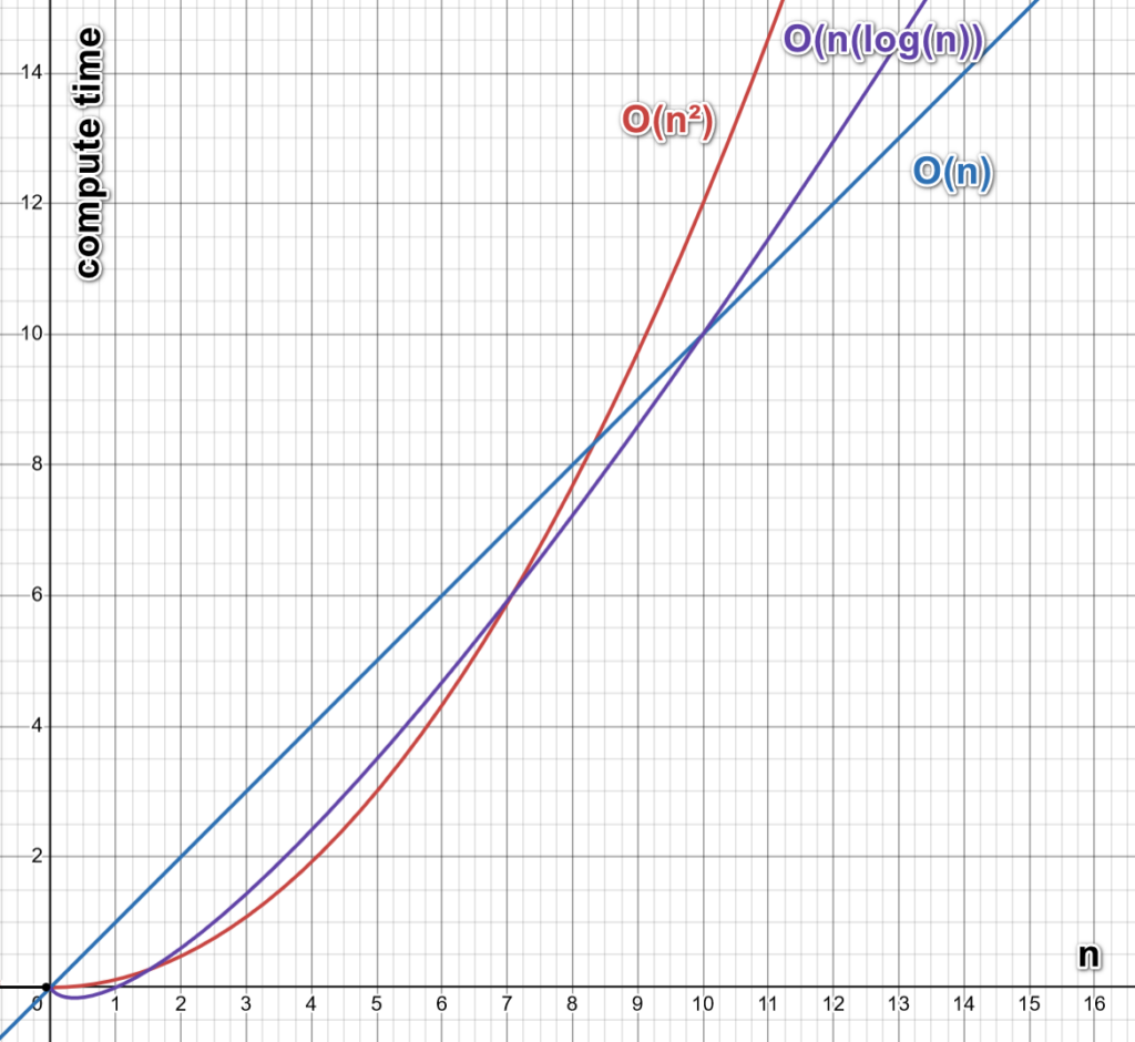
Algorithms are very often judged based on their “complexity.” What does “complexity” mean? Let’s take an example. For example, the time required to run a classical sorting algorithm (such as “HeapSort”) is proportional to “n log(n),” with “n” being the number of items to sort. In such a situation, we’ll say that the complexity of the “heapsort” algorithm is “O(n log(n)).”. All these concepts are illustrated in the chart here below:

A better sorting algorithm that is more environmentally friendly than the “HeapSort” would have a linear complexity that is noted: “O(n).” Linear complexity is faster and thus better because “O(n) < O(n log(n)).” In the context of the sorting algorithm, such a linear complexity (“O(n)”) is very uncommon (e.g., it’s not found inside the common data solution: Spark, R, Python, JS, Postgres, Oracle). It’s only found in a handful of software solutions, including Matlab and TIMi. When using TIMi, in some specific but common situations, the users can also decide to use another, even better, sorting algorithm with a “O(1)” complexity (this is unique to TIMi).
Regarding the algorithm used to compute “aggregations” (a very common operation in the field of Big Data), all big data solutions typically use an algorithm based on either a “hashtable” algorithm or a “B tree” algorithm. The complexity of an aggregation operation that is based on a “B tree” algorithm is very, very bad: “O(n² log(n))” with “n” being the number of rows to aggregate. The complexity of an aggregation operation based on a hashtable algorithm is better: it’s between “O(n)” and “O(n²)”. Unfortunately, the true observed complexity of the hashtable-based algorithms in the field of Big Data is nearly always approaching “O(n²)” (due to a large number of “collisions” inside the hashcodes because of the large data volumetry).
Amongst all big data solutions, TIMi is the only one to provide an algorithm to compute aggregations with a guaranteed complexity of “O(n)”. This guarantees a more efficient and faster aggregation, making the TIMi solution much “greener” than its competitors.
Let’s now talk about another very common operation in the field of Big Data: the “join” operation, that is used to join two tables (here below named T1 and T2). Big data solutions are using algorithms to perform “join” operations that have a complexity that is typically between “O(n1 log(n2))” and “O(n1.n2)”, where “n1” is the number of rows of the table T1 and “n2” is the number of rows of the table T2.
Amongst all big data solutions, TIMi is the only one to provide an algorithm to compute join with a guaranteed complexity of “O(n1+n2)”. In some specific but common situations, TIMi’s users can also decide to use another join algorithm with complexity “O(n1)”. This guarantees a more efficient and faster join than all other big data solutions, making the TIMi solution much faster and thus much more energy efficient than its competitors. Less energy consumed directly translates to a lower carbon footprint.
Optimized Implementations
In the previous paragraph, we introduced the notion of “complexity.” This is a very important and insightful notion when evaluating the quality of algorithms and software in general, but it can sometimes be misleading.
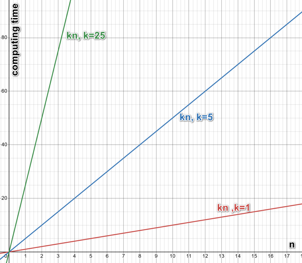
For example, let’s talk again about the algorithms used for “aggregation” operations. The complexity of the TIMi’s algorithm is guaranteed to be “O(n),” and the complexity of the “hashtable” algorithm (in a very favorable situation on a small table) is also “O(n).” What does this mean? It means that the running time to compute the aggregation is simply proportional to “n” (where “n” is the number of rows to aggregate”), or, in other words, the running time is “k.n” (where “k” is a constant value that is named the “constant term”). This concept is illustrated in the chart here below:

This “constant term” k changes from one algorithm (and one implementation) to the other. One very important and notable difference between two software resides in the value of the “constant term” k (that must be as small as possible). Inside TIMi, the different codes that are used to implement all the algorithms are written using low-level assembler code (and low-level, close to the metal, “C” code) to get “k” as small as possible. Almost all other big data solutions rely on a slow programming language (java, scala, python) that imposes a very high “k” value.
So, to summarize, at first view, the algorithms implemented inside TIMi (for aggregations) seem to have approximatively the same speed as the other implementations found inside other big data solutions since all these algorithms have, at least on paper, more or less the same complexity “O(n)”.
But, in practice, the “aggregation” algorithm implemented inside TIMi is several orders of magnitude faster than other implementations found in other big data solutions because of the much smaller “constant term” k found inside TIMi’s implementation. The same reasoning holds for all other algorithms (e.g., for sorting and joining tables) commonly found in big data solutions.
Distributed Computing
Distributing data processing tasks across multiple nodes can, some time, reduce the running-time of the most common operations found in big data (e.g. aggregations, join, sort). Some Frameworks such as Apache Hadoop, Databricks, Redshift, Snowflake and Spark are designed to execute the most common big data operations using many nodes.
The software architects that designed these solutions spent the vast majority of their time designing the architecture of these solutions to always be able to use all the nodes inside a cluster. The idea was to favor to the maximum what is commonly called “horizontal scalability”. Or, in other words, the idea was to have a software architecture that runs faster each time you add one more node/server.
This also means that, in comparison, practically no efforts were made to improve “vertical scalability” (i.e., no efforts were made to get the best algorithms and implementations while running on one single node/server). This very obvious lack of interest in “vertical scalability” might explain why TIMi is several orders of magnitude faster than all other big data solutions when running on one single node.
One very important notion when estimating the quality of a distributed computation engine is the “incompressible running time”. Let’s take a quick “deep dive” into this notion. If you want more information on this subject, please refer to the Wikipedia page on Amdahl’s Law. The implications of the Amdahl’s Law are also explained inside this Youtube video that compares the speed performances of Spark versus Anatella.
Let’s assume that you need to run some (distributed) computations on a cluster of machines. These computations are divided into two parts. The time required to execute this first part is named the “compressible time”: i.e., each time you add a node inside your cluster, this “compressible time” gets reduced (i.e., it gets “compressed”). On the other hand, the second part is named the “incompressible time”: it is a constant duration that does not change when you add more nodes inside your cluster of machines.
In an infinite infrastructure with an infinite number of nodes, the “compressible time” is reduced to almost zero while the “incompressible time” always stays the same. The “incompressible time” is typically expressed in percentage with respect to the running time on one node.
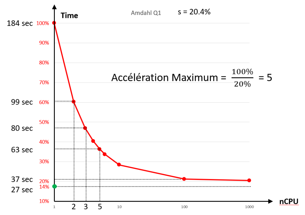
For example, an “incompressible time” of 20% means that, on an infinite infrastructure, the computing time is reduced to 20% of the computing time on a single node. In such a situation (with an “incompressible time” of 20%), thanks to the “distributed” computations, we get a maximum speed-up of “5” (=100%/20%) on an infinite infrastructure. In other words, the distributed computations are 5 times faster than the computation on a single node. This concept is illustrated in the chart here below:

(20% incompressible time) (The green dot is Anatella on 1 cpu)
When using a classical distributed framework, it’s very common to have “incompressible times” between 20% to 50% for the most common operations (for more details and numbers, see the “TIMi vs Spark TPC-H benchmarks” on Github or the academic paper titled “Amdahl’s law in Big Data: alive and kicking”). In some rare instances (such as computing very small aggregations with Teradata), the “incompressible times” can be reduced to 5%, but it’s very uncommon. It should be noted that, almost all the time, when using Databricks and Spark, the “incompressible time” is around 50%. What does this “50%” means in practice?
It means that, when using a very large infrastructure, with thousands of nodes, you will only achieve a speed-up of “2” (=100%/50%). In other words, the distributed computations on thousands of nodes are 2 times faster than the computations on a single node. From the point of view of energy consumption, it’s catastrophic: You are providing electricity and power to thousands of servers to get a speed-up of “2”. You are effectively polluting thousands time more, to get a speed-up of two.
How to get a higher speed-up? Higher than “2”? A possible solution to get a higher speed-up to solve all your big data problems would be to switch to TIMi. Indeed, one TIMi server is between 20 times to 102 times faster than a server running any other big data solution currently available on the market.
This is due to the deep focus of the TIMi’s team to achieve the highest “vertical scalability” possible (a technical choice that was not followed by any other current big data solution providers: i.e., these were only focusing on “horizontal scalability”). One possible explanation for the total disregard for “vertical scalability” and the utmost & total focus on “horizontal scalability” displayed by all these other big data solution providers would be the current enormous “hype” around cloud technologies.
Switching to TIMi running on a single node will effectively produce a speed-up between 20 to 102 compared to a poorly designed distributed computation engine (with a 50% incompressible time, such as Databricks, Spark, Redshift, and many others). Not only will your computation run faster, but at the same time, the energy consumption and CO production will be greatly reduced. The reduction on your CO emission is double because you are, at the same time, (1) reducing the hardware infrastructure to a single node and also (2) reducing the duration of the computations by a factor of at least 10.
It’s also possible to run distributed computations with TIMi. In such a situation, TIMi’s incompressible time is between 0% and 10%, depending on the operation. So, if you are an unconditional fan of distributed computations, TIMi is also one of the best solutions possible for you thanks to its very low “incompressible time”.
TIMi: Leading the Way in Sustainable Big Data
Founded in Belgium on August 3, 2007, by Frank Vanden Berghen, TIMi (The Intelligent Mining Machine) has been at the forefront of developing tools for efficient and sustainable big data processing. Initially known as Business-Insight SPRL, the company rebranded to TIMi on December 28, 2017. TIMi’s software suite, which includes Anatella, Modeler and Stardust exemplifies the principles of energy-efficient big data architectures.
TIMi’s Contributions to Sustainable Big Data
Anatella, TIMi’s core component, is designed for high-performance data transformation. Unlike general-purpose ETL (Extract-Transform-Load) tools, Anatella is optimized for analytical tasks. Thanks to a deep focus on vertical scalability, Anatella processes large datasets with minimal infrastructure. This efficiency translates to lower energy consumption.
Anatella’s performance was highlighted in a vendor-neutral benchmark, TPC-H, where a single Anatella node exhibited higher speed than a whole Spark-based cluster with hundreds of nodes. Another example of Anatella’s efficiency would be the benchmark organized by the “National Bank of Belgium” (the governmental institution that prints Euros in Belgium). Anatella running on a single 2000€ laptop completed this benchmark in 18 hours while the whole Databrick cluster from the bank, composed of hundreds of nodes, did run for 3 months (more details here).
TIMi Modeler is one of the first auto-ML (automated machine learning) tools available worldwide. Its design allows for scalable, energy, and resource-efficient machine learning operations. The TIMi Modeler reduces the computational load and energy required for model training and deployment by automating complex machine-learning processes.
Stardust, another critical component of the TIMi suite, excels in computing accurate clusters for large populations. This capability is crucial for sectors like telecommunications, where analyzing data from millions of users is commonplace.
Future Directions
The future of environmentally friendly big data architectures lies in continued innovation and the adoption of cutting-edge technologies. Advances in edge computing, algorithm innovation, and integrating renewable energy sources will play significant roles.
Environmentally-friendly architectures for big data are essential for sustainable development in the digital age. Companies like TIMi are leading the charge with innovative solutions that enhance efficiency and reduce the environmental impact of data processing. By leveraging advanced technologies and adopting sustainable practices, we can ensure that the growth of big data does not come at the expense of our planet.
Source : Reducing the Big Data Carbon Footprint with TIMi by The Washington Times


