36 additional models in 2 days

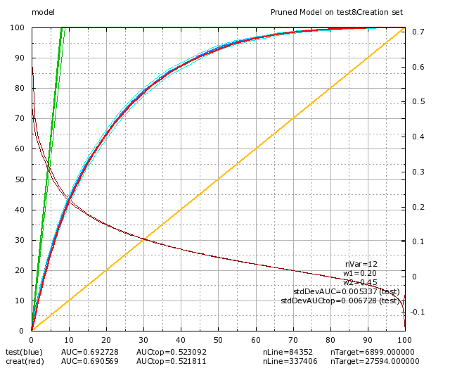
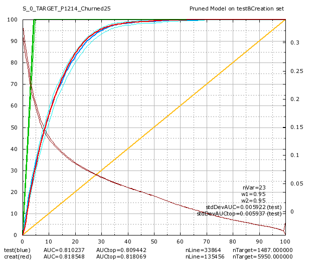
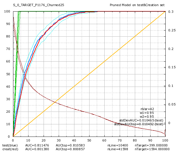
Colruyt was also interested in predicting a “partial churn”: A “partial churn” means that the customer continues to buy some product but there exists some categories of products were the customer has stopped buying anything. There are 83 product categories at Colruyt. Amongst these 83 categories, there are 47 categories that are very small and it makes no sense trying to predict anything for them. After two additional days, we got 36 additional models “per categories of product” (i.e. models for “partial churn”). Here are some of these models:

Data-transformation

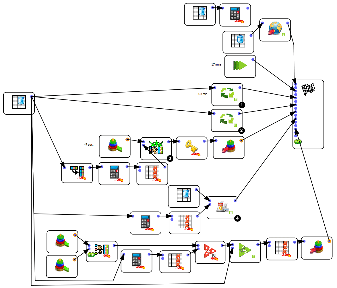
To build these models, we received a table (as a text file) where each row is: “a customer X bought the product Y at the date D”. This table has 1.4 billion rows (2 years data). Since the Anatella scripts are developed, the total computing time required to update the 36 models (starting from raw data) is around 1 hours. The data-transformation graph that was developed to create these 36 models from raw-data was:

Note  1 

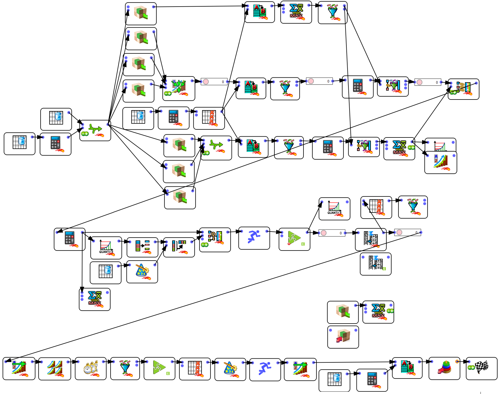This actually runs inside a loop a complex sub-procedure located in a sub-graph. At each iteration of the loop, we compute (using the sub-graph) a different “Target Column” (we have 36 targets to compute). The 36 computations are running in parallel on 16 cores (Anatella makes heavy uses of parallel and multithreaded computing). This sub-graph is:

Note  2 

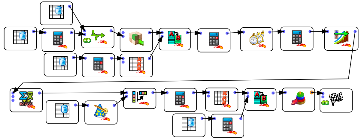This runs inside a loop a sub-procedure located in a sub-graph. Each run of the sub-graph computes 26 variables that are representing the consumption behaviours of each customer in a specific product category. Since, there are 36 product categories, Anatella produces as output 36 tables (with 26 variables in each). This subgraph is:

Note  3 

This makes a left-join between the “main table” (40 socio-demo variables), the 36 tables containing the 36 targets (computed during “note 2”) and the 36 tables computed during the previous step (“note 3”). This left-join involves thus 1+36+36=73 tables. The output table has thus 40+36×26+36×1=1012 columns and 660K rows. On a $1000-laptop, the computation time for the left-join is 9 seconds (this is several magnitude faster than any other solutions). In opposition to other tools, Anatella has no limitation on the number of tables inside a join operation and on the number of columns involved inside a join operation. Anatella is also several orders of magnitude faster than any other software.

Note  4 

This box is a model factory: it automatically creates “in batch” the 36 required models based on the unique table computed during “note 3”. To remind you, the dataminers from Colruyt attempted to create one such model for 2 years.