Controlling Model Drift With Timi Modeler

Timi modeler is a great tool to get models fast. It doesn’t mean they have to be “rough” or ‘inaccurate”. With its default settings, Timi modeler allows citizen data scientists to have, very quickly, a robust model that will have an incredible lift, and identify properly the key variables, and will do a very good job to control over-fitting.

Over-fitting is the general problem that occurs when models explain “too well” a training dataset, but only generalize poorly when applied to other datasets. By relying on K-Fold cross-validation and the usage of learning, test and validation samples, Timi does a good job at this. Mathematically.

However, the world is not mathematics. and when it comes to “good” models, the key differentiator is more often the analyst (you), than the algorithm or tool that you are using. Some tools, however, make it easier for you to be brilliant.

There is one general rule to apply when generating a model: if you can’t explain it, fix it! A second rule is that lift, AUC or Gini are not the most important things: model stability is. In other words, it’s much better to have a slightly lower lift, but consistent over time. For example, if you use a tree algorithm (like C5) and specify parameters to get very small terminal nodes, you will have a very good lift, in a terrible model overall.

If you build a model with the Census Income 94-95 database (installed with Timi) you will see that some variables in the model show a strange behavior.

Let’s explore Capital Gain

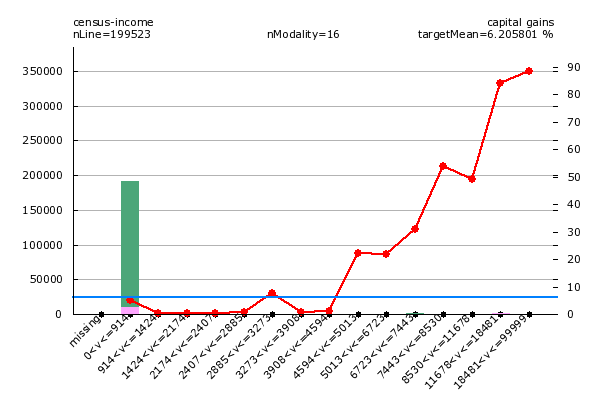
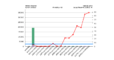
This chart shows two strange things: supposedly, the likelihood to have to pay taxes decreases for capital gains over 91 USD, and then only increases after 4.600 UDD. Unless you make between 2.885 and 3.273 USD. In this case, you are more likely to have to pay income taxes. And if you make a lot of money, the “safe zone” is between 8.530 and 11.678 USD.

This is obviously horse poop. Mathematically validated horse poop.

There are two strategies that can help fix this: a “cheap” one, and an “expensive” one.

Cheap control of overfitting

Make bigger categories. In the Modality recoding, you can globally set the bins for all variable, the largest the bin, the lowest the risk of drift. And the less precise the model. This is where talent comes in: when you find a great way to cut a particular variable, you get a better model:

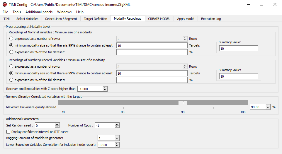
Still, a one-size-fits-all approach rarely works in data mining. Which is why it’s a much better idea to control this at a variable level. In the variable selection tab, you will find an additional tab: discretization / penalization. This allows you to set the binning parameters of a particular variable without affecting the rest of the dataset:

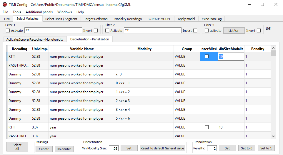
This was the “cheap” way to do it. Why cheap? it actually makes the model building FASTER!

Expensive control of overfitting

Another way to deal with it is to set a constraint of monotonicity on a variable. for example, consider that a higher income should ALWAYS mean higher probability to pay income taxes. This option is available in the variable selection tab:

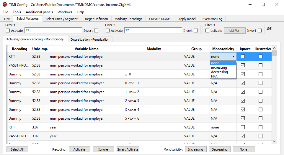
This will not affect how bins are created, but this will set a constraint on the shape of the variable’s distribution.