<< Click to Display Table of Contents >> Navigation:  5. Detailed description of the Actions > 5.13. TA - R_Discovery Analytics > 5.13.6. Latent Class Analysis Clustering ( action)

 

Icon:  

 
Function: R_poLCA
 

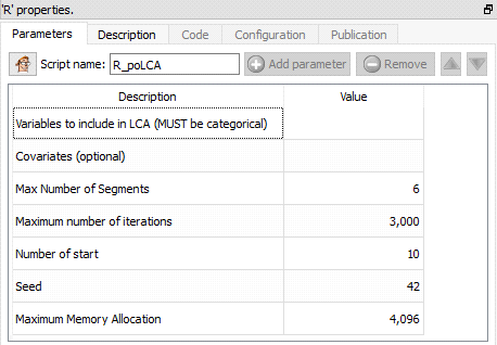
Property window:

 

 

Short description:

 

Latent Class Clustering.

 

Long Description:

 

This Action is mainly for explanatory/teaching purposes. If you want to create a better segmentation, you should use Stardust.

 

Variables must be ordinal, with few categories, on TINY dataset!

 
The code is mosty inspired from http://statistics.ohlsen-web.de/latent-class-analysis-polca/

 

Latent Class Clustering is a method that allows to group categorical variables more efficiently and has the advantage of providing measures of goodness of fit. For more information about the fundamentals of it, I invite you to read the works of Magidson and Vermunt who developed the method.

 

The key advantage is that it takes the shape of distributions into account, and mixes them (hence the other name: Finite Mixture Models). It is often presented as a probabilistic extension of K-Means, although it has a completely different objective.

While K-Means attempts to maximize external homogeneity (we want centers as far from each other as possible) and internal homogeneity (we want the observations in our segments to be as similar as possible), Latent Class looks for a latent variable that explains why local independence is not respected.

 

What is local independence? Let’s consider a simple example: users of facebook vs users of LinkedIn.

If the two variables were independent, the probability to use one facebook and MySpace should be the product of the two probabilities. Remember this concept: . In this case, we should have 40%*50%=20% of the population using Facebook and MySpace.

 

 
 
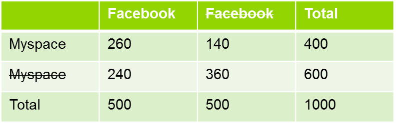
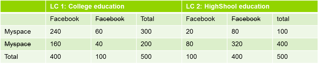
Clearly, this is not the case. There has to be something that explains it. This something else is what Latent Class is looking for, an unobserved variable that cuts the population in such a way that our equation holds true.
 

 

 
In their publications, Magidson and Vermunt concluded that LC performs as well as DISC, and better than k-means in terms of classification errors when working with known classification dataset. Besides this, Latent Class has many advantages vs K-Means:
 

•Probability-based classification, which performs better than distance based classification, gives goodness of fit indication (BIC is to be preferred to AIC) and includes indicators of statistically optimal number of clusters

•No need for standardization of variables (scale independent)

•No assumption of normality and homoscedasticity, it actually allows a combination of mixed scales: continuous, ordinal and nominal variables.

•Local independence (segments are not correlated).

•Covariate based profiling (no further analysis needed for discrimination).

 
Currently, this technique is not included in Stardust (as is does not work with hundreds of thousands of records).

 

There are three main software packages that include the implementation of Magidson and Vermunt: Latent Gold (the original one, and in our humble opinion, the best one), SAS, and – of course - R.

 

 
 
First, you need to sample. 2000 is a lot, 5000 rows is big Data, 10.000 rows is hours of computation, 20.000 is probably going to crash. Remember this is distribution based, so designed to work with samples of 20-400 records per segments.
 

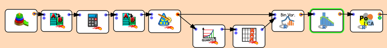
Then, there are a few operations in data transformation that are required before you can run Latent Class
 

1-Rename variables (remove spaces and special characters)

2-Bin variables: you need to recode your variables to a small amount of levels (ideally 3-5 levels max)

 
Then, simply select the recoded variables in PoLCA, and click on the SECOND OUTPUT PIN to get a feeling of model quality
 

 
 
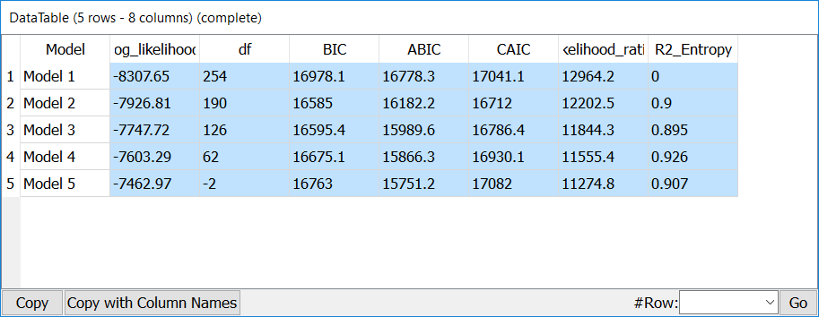
The most important metrics here is BIC, which should be as small as possible, but with positive degrees of freedom.

 

In this case, the optimal BIC is a 2-cluster solution, while R2 Entropy suggest an optimal solution at 4 segments. As there are really very little degrees of freedom for this solution, our instinct would be to stay at 2 segments… but still explore all of them,

 

The first output pin gives us the solution for each model
 

 
 
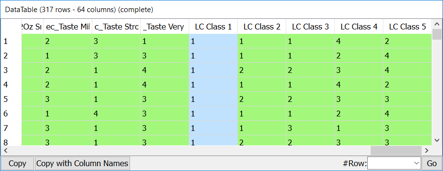
It is therefore quite easy to simply get a few transition tables and study what information is gained by each model.