To explain how to use the PCA technique to do « dimentionality reduction », we will start with a small example. We have here many points in 2D (2 dimensions) and we want to reduce the dimension to 1D:
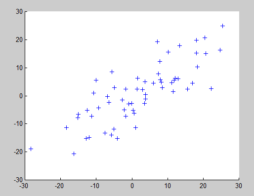
(For the census-income database, we have points in 7D and we want to reduce the coordinates in 3D).
The output of the PCA analysis is a set of different perpendicular directions represented in red on the chart below:
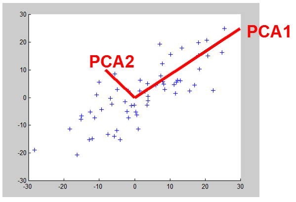
Let’s project all the blue points of the database on the first PCA axis (PCA1): the projection is illustrated in this chart in green:
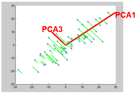
We obtain a new dataset that is represented here in blue:
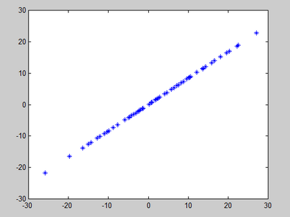
This new dataset can be “seen” in one dimension along the PCA1 direction:
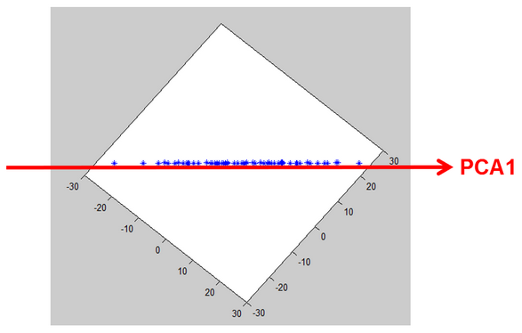
We just reduced the dimension: the 2D points are now in a one-dimensional-space. During the dimensionality reduction, we didn’t lose too much information because the distance between the (same) point “before” and “after” projection is small. This is thus a good dimensionality reduction.