<< Click to Display Table of Contents >> Navigation:  5. Detailed description of the Actions > 5.13. TA - R_Discovery Analytics > 5.13.3. K-Means Clustering ( action)

 

Icon:  

 
Function: R_KMEANS
 

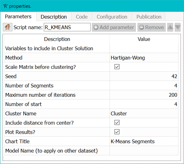
Property window:

 

 

Short description:

 

K-Means Clustering.

 

Long Description:

 

This Action is mainly for explanatory/teaching purposes. If you want to create a better segmentation, you should use Stardust.

 

The K-Means algorithm is the most commonly used clustering/segment algorithm used everywhere. If you search for a good starting point to start segmenting your data, use the K-Means algorithm.
 

The Kmeans action will output a new column with the cluster number, and columns with the distance between each point and the center of each segment. You can easily transform this information into probability.

 

The K-Means algorithm has several advantages agains hierarchical clustering. To being with, it will work on large amount of data at a more reasonable speed. It also allows observations to switch group as cluster centers are recomputed. These advantages made K-Means the most popular segmentation method, but the K-Means algoritm has sevelar limitations:
 

1.it assumes all variables are continuous, identically distributed, and belong to spherical segments of equal variance (this is probably the most limiting hypothesis)
 

2.it assumes that all variables are on the same scale. While this is problematic, this is easily circonveined by normalizing the data or simply selecting the option “scale matrix”

3.it assumes that all axises (i.e. all variables) are non-correlated. You can check the correlations that exists between the variables using the covariance action (see section 5.7.11). You can easily obtain non- correlated variables (i.e. perpendicular axises) by running the k-means algorithm inside the space spanned by the first “Principal Component Axises” (i.e. the first PCA’s). Since is why, most of the time, you should (nearly always) use a PCA action (see section 5.12.7) before the K-Means action.
 

4.It does not accept any non-numerical variables
 

5.The number of clusters (k) must be known before hand. It is therefore often used in combination with hierarchical (ward) clustering (to find the correct value for k).

 

 
Algo: Method:

 
In most cases, H-W is used. However, all other algorithms are available.

The algorithms used inside this Action are described in the following papers:
 

•Forgy, E. W. (1965) Cluster analysis of multivariate data: efficiency vs interpretability of classifications. Biometrics 21, 768–769.

•Hartigan, J. A. and Wong, M. A. (1979). A K-means clustering algorithm. Applied Statistics 28, 100–108.

•Lloyd, S. P. (1957, 1982) Least squares quantization in PCM. Technical Note, Bell Laboratories. Published in 1982 in IEEE Transactions on Information Theory 28, 128–137.

•MacQueen, J. (1967) Some methods for classification and analysis of multivariate observations. In Proceedings of the Fifth Berkeley Symposium on Mathematical Statistics and Probability, eds L. M. Le Cam & J. Neyman, 1, pp. 281–297. Berkeley, CA: University of California Press.

 
 

Parameters:

 
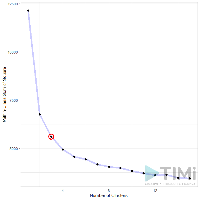
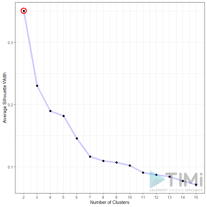
ALGO: WSS optimal Number Selection: use the elbow method or the WSS to select the optimal number of segments. While a visual selection with Hierarchical is often preferred, those two methods offer an alternative selection of the number of segment. The Elbow method selects the inflection point of the Within Sum of Square line, while the silhouette method is defined as follows:
 

“Put a(i)= average dissimilarity between I and all other points of the cluster to which I belong.

(if i is the only observation in its cluster, s(i)=0 without further calculations). For all other clusters C, put d(i,C) = average dissimilarity of i to all observations of C. The smallest of these d(i,C) is b(i)=minCd(i,C), and can be seen as the dissimilarity between i and its “neighbor” cluster, i.e., the nearest one to which it does not belong. Finally,

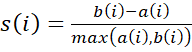
Observations with a large s(i) (almost 1) are very well clustered, a small s(i) (around 0) means that the observation lies between two clusters, and observations with a negative s(i) are probably placed in the wrong cluster.”1
 
 

ALGO: Scale Matrix before clustering: proceed with a normalization of the data to avoid dominance from varaibles on a larger scale.

ALGO: Seed: set a seed number so you can run the same analysis again, with consistent results.

ALGO: Number of segments: Select the number of segments to keep.

ALGO: Number of iteration: set stopping criteria in case of no convergence.

ALGO: Number of starts: How many random sets are chosen.

OUT: Cluster Name: name of the variable with the cluster results.

ALGO: Include distance from center: include Euclidean distance from centers as new variables.

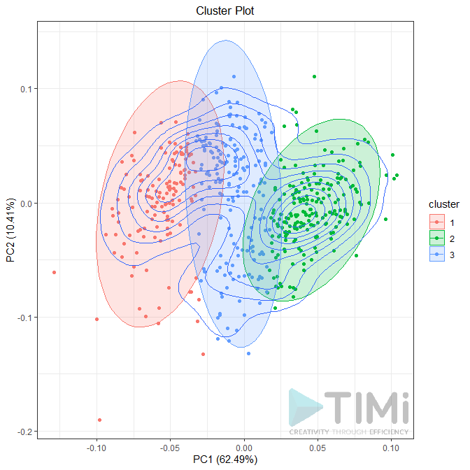
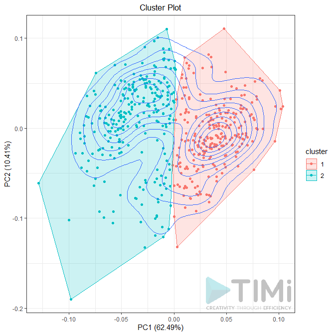
CHT: Plot Results: Select whether or not to display a distribution chart

CHT: Chart title: set the title of the chart (if you selected the previous option)

CHAT: Cluster Border: Limites or Ellipse.

 

 

Model Name: Name of the model to use for later scoring.