<< Click to Display Table of Contents >> Navigation:  5. Detailed description of the Actions > 5.13. TA - R_Discovery Analytics > 5.13.2. Hierarchical Clustering ( action)

 

Icon:  

 
Function: HIERARCHICAL
 

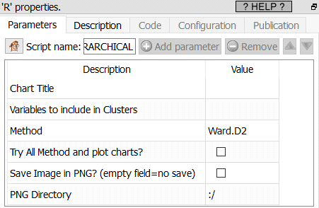
Property window:

 

 

Short description:

 

Hierarchical Clustering.

 

Long Description:

 

This Action is mainly for explanatory/teaching purposes. If you want to create a better segmentation, you should use Stardust.

 

A classic algorithm that always works, as long as data is numerical and not too big.

 

Typically, hierarchical clustering is used in combination with K-Means, to find the optimum the number of segments. In general, it is not recommended to trust segments assignments made by hierarchical clustering.

 

The main limitations of Hierarchical clustering are:
 

•it needs to start by computing the distances betweem each point, hence creates an n x n matrix in memory. This will not work with “large” database (1000 records are ok. 10.000 is often a problem. 10.000 will require a large server with a LOT of ram)

•Curse of dimensionality: if you put a lot of variables, segments will not appear (everything will look equidistant)

•it is slow

•cluster centers are not dynamic: as we regroup, centers change and some points may become misclassified

 

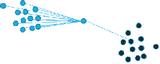
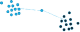
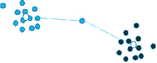
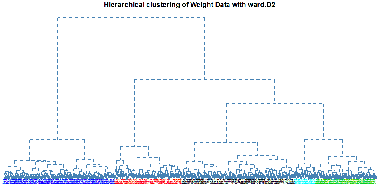
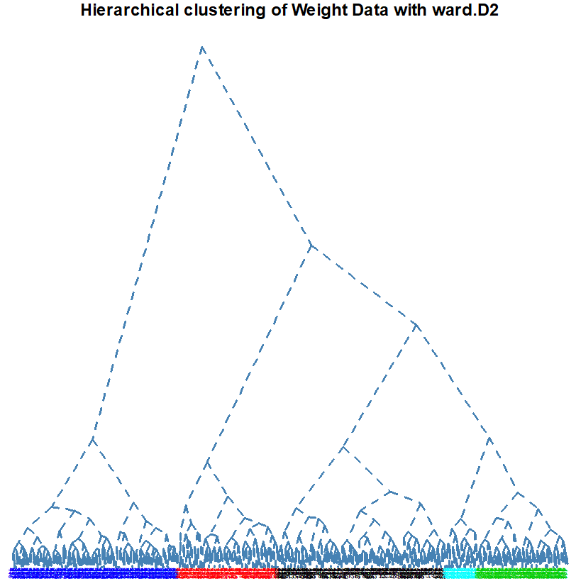
While several methods are included in this action, it is best to used Ward.D2: This is the same distance estimation used in other popular statistical software (Stardust, SPSS, etc.), and it tends to give the clearest dendograms: compare Ward with Average Linkeage method: The latter tends to create segments of outliers and fails to provide a clear cut un terms of number of segments.

 

 

 

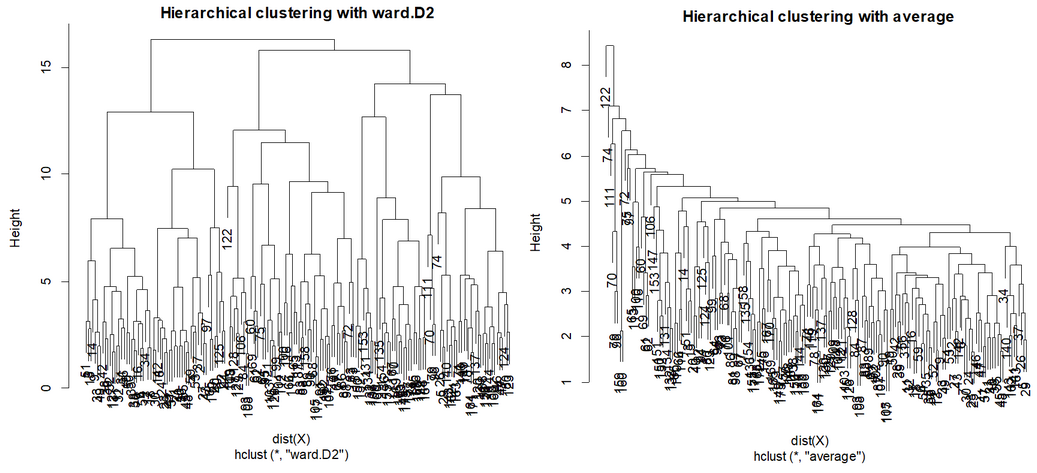
To know how many segments to retain, one must “look for a large drop of information”, and explore the solutions of the various potentially “good” solutions.

 
Parameters:
 

Chart Title: Title of the plot. It will display “Hierarchical Clustering of “ TITLE “ with METHOD”
 

Variables to include in Clusters: select the columns on which to compute the clusters
 

Method: choose one of
 

Ward.D: Ward’s distance, Minimize the total variance of the clusters. Proximity between two clusters is the magnitude by which the distance in their joint cluster will be greater than the combined distance in these two clusters: SS12−(SS1+SS2)
 

Ward.D2: Squared Ward’s distance (the most common one), we use the sum-square instead of the distance
 

Single: Single Linkage follows the logic of “a friend of a friend is a friend”, in which points are assigned to the segment with the closest point

 

 

 

Complete: Complete linkage follows the logic of “the one I hate the most is my friend”, points are assigned to the segments that have the least distant extreme, that is, the farthest point is the closest.

 

 

Average: Average Linkage: we take the average distance of all points for all clusters, weighted by the number of points in each cluster.  You’d expect good segments, they are often not that clear.

 

 

Mcquitty: average, without the weight.
 

Median: (WPGMC) Similarity based on the median of each cluster (similar to K-Medoid) using Euclides’ distance

 

 

Centroid: UPGMC, distance to the center of each cluster using Euclides´s distance.

 

 

 

Direction: Select:

 Downwards

 Upwards

 Left

 Right

 
Try all methods and plot chart: run all method so we can choose which is best, visually
 

Save image as PNG: self explanatory
 

PNG Directory: specify the directory in which to save the PNG, the name will be the plot title
 

Row Labels: mandatory, select the variable with labels names, it can be the key.
 

Label Size: label size on the plot
 

Line Type:
 

 
 
Dendogram Type:

 

 

 

 

 

 

 

 

 

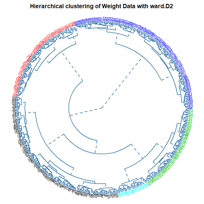
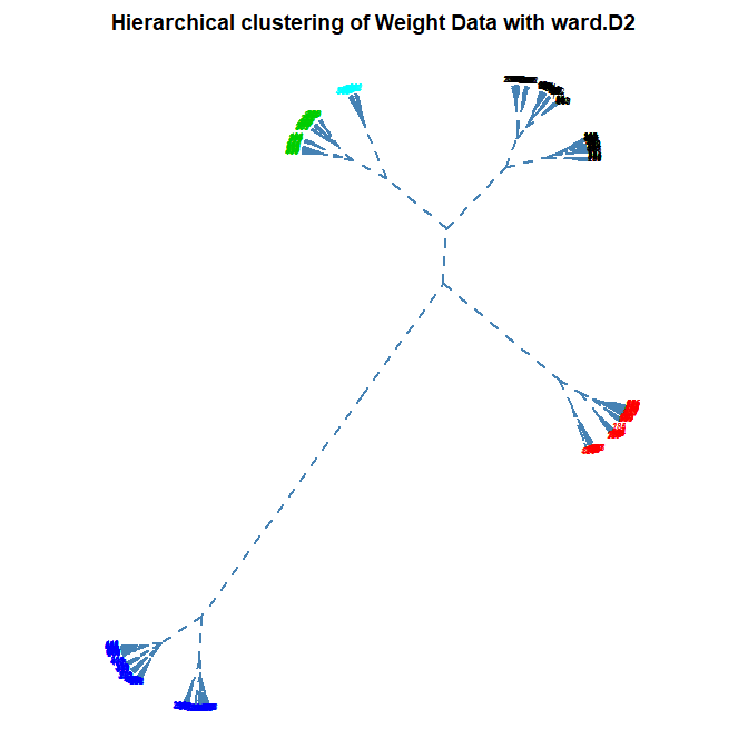
Number of Clusters: set the number of clusters to display in color on the plot (default is 1)
 

Cluster Name: name of the cluster