<< Click to Display Table of Contents >> Navigation:  5. Detailed description of the Actions > 5.12. TA - R Predictive > 5.12.2. CART – Step 1 - Create one “deep” tree ( action)

 

Icon:  

 
Function: My_R_CART_Full
 

Property window:

 

 

Short description:

 

Create a tree using the CART algorithm.

 

Long Description:

 

The CRT node uses Recursive Partitioning and Regresion Tree as implemented in the R rpart library, based on the 1984 book of Breiman, Friedman, Olshen and Stone. The library is the work of Terry Therneau, Beth Akinson, and Brian Ripley.

 

A complete introduction to the technique can be found in:

https://cran.r-project.org/web/packages/rpart/vignettes/longintro.pdf

 

This generates a CART model, and send the following output tables:
 

Output pin 0 : full table with prediction

Output pin 1: error table for selection of pruning parameters

Output pin 2: variable importances

Output pin 3: Saved Model Name

 

The goal of this analysis is to generate a large tree and identify where to prune it (see next action node). While this algorithm has gained popularity in the early stage of data mining, it is now increasingly being left unused.

 

The main advantage of CART is it ability to combine nominal and continuous variable to predict (typically) nominal groups. Being non-parametric, it adapts to fairly large datasets, and does not suffer from multicollinearity or non-normality of the data. When it was introduced, it was also highlighted that it yields better predictions than CHAID.  Another key advantage is that it is intuitive, and offers a methodology similar to a drill down, but with some validation.

 

The key problems of CRT are that as trees deepen, we are almost certain to overfit the data (some argue that trees below three levels should mever be used, other go up to 6 or 7 levels). Indeed, as we see a succession of conditional probabilities, whatever comes out of the model becomes irrealistic, which is why many use combinations of hundreds of small trees (XGBoost, TreeNet, Forest of Stumps, etc.) to overcome this problem. This yields better models, but they are “black boxes”.

 

In practice, the first cut is often based on particularities of the sample, and the following cuts are dependent on the first one, making such models unstable for predictive purposes. They are, however, useful in terms of data exploration and understanding.

 

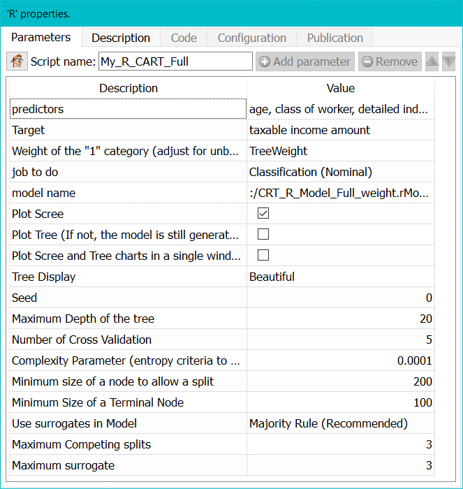
Parameters:
 

The CRT tree (Classification and Regression Tree) requires the following settings:
 

Predictors: list of independent variables we want to use to predict in the form of x1+x2+…+xk

Target: the variable we want to predict (binary, continuous, or multinomial)

Weight: the tree needs to be “balanced”, so it is a good idea to create a weight variable. If all categories are equal, this variable is a constant. Usually, use (1/apriori) for records with a target 1, and 1 for records with 0.

Job to do: classification or regression

Model Name: name of the model file. This is required to add pruning, or apply the model as is.

Show Plots: unselect this option to avoid showing any plots (run model without visual information)

Plot Scree and autoPrune: select whether to plot the Scree Plot to identify where overfitting begins. You can also set an automatic pruning based on minimum error or “elbow” method. Elbow will yield smaller, often more stable trees.

Plot Tree: select whether to plot the treee

Plot Scree and Tree chars in a single window: self explanatory

Tree display: simplified or fancy. The simplified one is much faster to display, but will not show text categories properly.

 

 

Advanced Parameters:
 

Seed: set a seed value to be able to change the starting point, or reproduce a previous model

Maximum depth of the tree: set how many successive splits are allowed. Note that very deep trees are unstable (overfitting). Typically, more than 10 is not worth exploring. More

Minimum size to allow a split: crt weill not cut nodes than have less observations

Minimum size of a terminal node: when splitting, CRT will attempt to respect this size. If splitting a node leads to a terminal node smaller than this criterion, the split will not happen

Use surrogates in model: this option allows you to control what happens in case of missing value.

•Display Only: an observation with a missing value for the primary split rule is not sent further down the tree.

•NO Split for all missing: means use surrogates, in order, to split subjects missing the primary

•variable; if all surrogates are missing the observation is not split.

•Majority Rule (recommended): if all surrogates are missing, then send the observation in the majority direction. This corresponds to the recommendations of Breiman et.al (1984).

Maximum Competing Splits: the number of competitor splits retained in the output. It is useful to know not just which split was chosen, but which variable came in second, third, etc

Maximum Surrogate: the number of surrogate splits retained in the output. If this is set to zero, the

compute time will be reduced, since approximately half of the computational time (other than setup) is used in the search for surrogate splits. However, this will yield to a model harder to put into production.

 

In the log, you will see the details of the analysis. The Scree plot shows the shape of the error reduction (and gives you a pruning criterion):

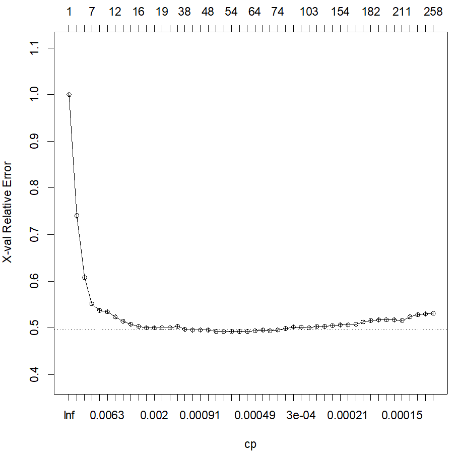
Once we observe a flat line, there is no improvement on the relative error, hence the tree is most likely overfitting by creating additional cuts. In the log, we can see details of this metric, where we see that two “good” stopping criteria could be 18, where it seems to stabilize, or 47 splits, based on the minimum error:

 

 

 

A chart with variable importance is also returned:

 

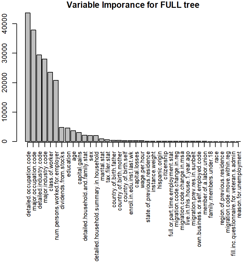
You will also find this information in text format in the Anatella log-window.