Icon: ![]()
Function: tesselateGIS
Property window:
Short description:
Tesselate the plane
Long Description:
To contruct some POLYGONs from POINTs inside Anatella, you can either use the ![]() tesselateGIS action or the
tesselateGIS action or the ![]() ConcaveHullGIS Action.
ConcaveHullGIS Action.
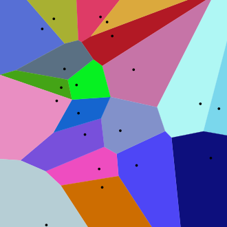
The general principle of the ![]() tesselateGIS is the following: It divides the plane into many small (convex) POLYGONs. The input of this Action is a set of POINTs that are named “Seeds”. For each seed, there is a corresponding POLYGON, called a Voronoi cell, consisting of all the points in the plane that are closer to that seed than to any other seed.
tesselateGIS is the following: It divides the plane into many small (convex) POLYGONs. The input of this Action is a set of POINTs that are named “Seeds”. For each seed, there is a corresponding POLYGON, called a Voronoi cell, consisting of all the points in the plane that are closer to that seed than to any other seed.
Here is an illustration:
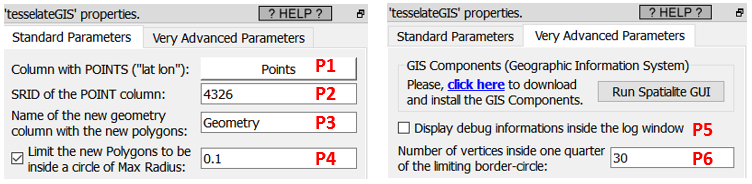
The ![]() tesselateGIS action uses an algorithm named “Voronoi diagram”. Unfortunately, these “Voronoi diagrams” are ill-defined on the border of the map: i.e. when we refer to the the “basic” definition of a Voronoi cell (i.e. the convex geometries given as the output of this Action), we see that these cells are not finite on the border of the map: i.e. They extend to the infinity. To avoid infinite geometries, Anatella limits the size of the cells to a disc centered at the seed of each cell. The radius of this disc is defined using the parameter P4. The number of points defining each disc is the parameter P6 multiplied by 4.
tesselateGIS action uses an algorithm named “Voronoi diagram”. Unfortunately, these “Voronoi diagrams” are ill-defined on the border of the map: i.e. when we refer to the the “basic” definition of a Voronoi cell (i.e. the convex geometries given as the output of this Action), we see that these cells are not finite on the border of the map: i.e. They extend to the infinity. To avoid infinite geometries, Anatella limits the size of the cells to a disc centered at the seed of each cell. The radius of this disc is defined using the parameter P4. The number of points defining each disc is the parameter P6 multiplied by 4.
The typical usage of the ![]() tesselateGIS action is to create “catchment area” for your shops. To do so:
tesselateGIS action is to create “catchment area” for your shops. To do so:
•You use as “seeds” (as input of the tesselateGIS action) the position of your shops.
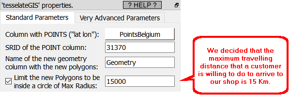
•You define the maximum distance that a customer would deem reasonable to travel to your shop using the parameter P4.
..and then you run the ![]() tesselateGIS action. Then, you can look at your “catchment area” for each of your shop: Just follow the procedure given in section 5.10.9.3: This section contains this exact example about displaying “catchment areas” for your shops.
tesselateGIS action. Then, you can look at your “catchment area” for each of your shop: Just follow the procedure given in section 5.10.9.3: This section contains this exact example about displaying “catchment areas” for your shops.
This ![]() tesselateGIS Action assumes that all your geometries are defined in a standard PLANAR coordinate system (i.e. not inside the SRID 4326), so for best results, you shouldn’t use it inside the SRID 4326 (i.e. use the
tesselateGIS Action assumes that all your geometries are defined in a standard PLANAR coordinate system (i.e. not inside the SRID 4326), so for best results, you shouldn’t use it inside the SRID 4326 (i.e. use the ![]() ReprojectGIS action to do all computations in a better SRID).
ReprojectGIS action to do all computations in a better SRID).
Here is a complete project, from start to finish, to create a “catchment area” for each of your shops:
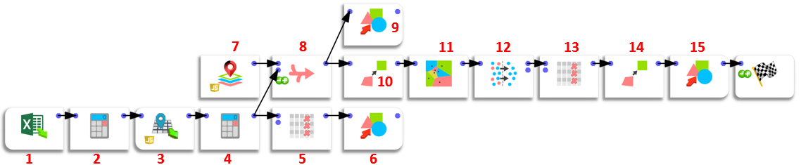
Here is a small description of each of the steps (illustrated with a RED NUMBER in the Anatella graph here above):
1.Extract the postal address of each of you shops from an Excel file.
2.Compute an “address” column that is the concatenation of StreetName, StreetNumber, Zip code, Town, Country
3.Use BING to find the Latitude and Longitude of your shops, using the “Address” column that we just defined during step 2 (see section 5.10.4 for more details about the ![]() bingMapGeocode action).
bingMapGeocode action).
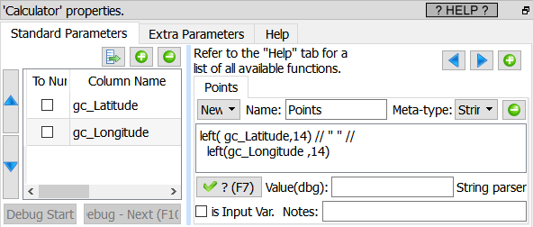
4.Create a “POINTS” column that is the concatenation of the columns “gc_Latitude” and “gc_Longitude” originating from BING. This column contains the “seeds” that we will send to the ![]() tesselateGIS Action to compute the “catchment areas” for your shops.
tesselateGIS Action to compute the “catchment areas” for your shops.
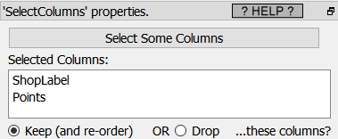
5.We want to create a .shp file with all the coordinates of all our shops (we do that in step 6). The first column of the .shp file contains the “label” of each point/shop. We use the selectColumn Action to select a good “label” column as our first column inside the .shp file:
6.We create the “SHOPS.shp” file (see an example on how to use it inside the section 5.10.9.3.)
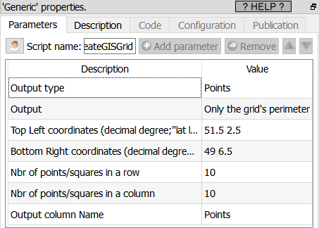
7.The ![]() tesselateGIS Action has the bad tendency to truncate geometries at the border of the map. So, we add some “artificial” points on the outline/border of the map (that we’ll remove during step 12) so that no geometry truncation happens for the “real” points that really represents our shops (that we obtained during step 4).
tesselateGIS Action has the bad tendency to truncate geometries at the border of the map. So, we add some “artificial” points on the outline/border of the map (that we’ll remove during step 12) so that no geometry truncation happens for the “real” points that really represents our shops (that we obtained during step 4).
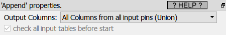
8.Create a new table with the “artificial” points on the borders (from step 7) and the “real” points (from step 4).
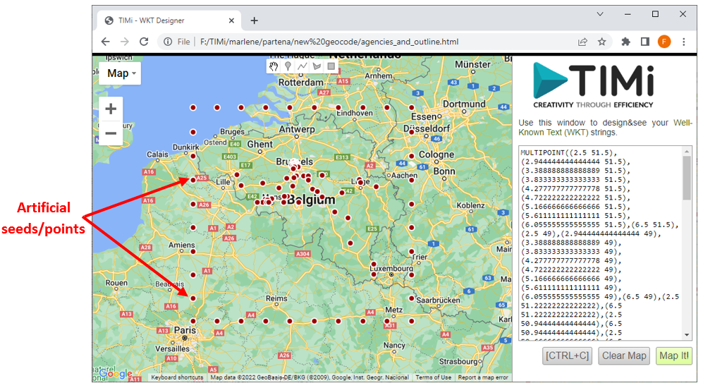
9. Validate visually the positions of the “artificial” seeds on the borders (from step 7) and the “real” seeds (from step 4):
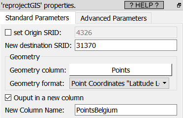
10.Reproject all the seeds defined in SRID 4326 inside the column “POINTS” to a new coordinate system (SRID 31370) which is the best for computation on Belgium. The new seed coordinates (inside the SRID 31370) are stored inside the new column named “PointsBelgium”.
11.Compute the Catchment Area for all the shops inside the SRID 31370 (because we used as “seeds” the column “PointsBelgium” that is in SRID 31370).
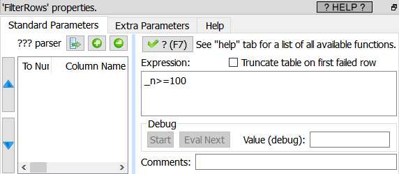
12.Remove the “artificial” seeds because we don’t need them anymore (i.e. remove the first 100 rows):
13.Remove/drop the column “PointBelgium” because we don’t need it anymore.
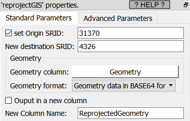
14.Reproject our geometries (i.e. our “catchment areas”) inside the SRID 4326 for visualization.
15.Save our geometries into the “SHOPS_ CATCHMENT_AREA.shp” shape file with the geometry column that contains the polygons that defines the catchment area for each shop. One row per shop.