The Ward’s algorithm has a strong limitation: it only works when the segments are spherical.
Let’s take a first example: we start from the 3 segments (Red, Green Blue) delivered by the K-Means algorithm:
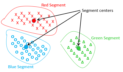
In the above graph, each cross, circle or triangle represents an individual.
Inside this first example, the centers of the red and blue segments are the closest centers, and thus one iteration of the standard ward’s algorithm will “group” together the red and blue segments inside a new (purple) segment, as illustrated here:
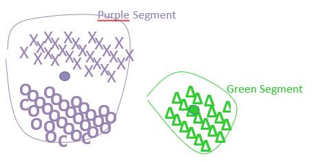
Please note that the center of the purple segment is at a completely new position that is the center of gravity of the all points inside the red and blue segments. On this first example, the Ward’s algorithm is working as expected.
Let’s consider a more difficult example (we did not represent the individual points anymore):
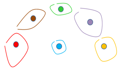
After 3 iterations of the original Ward’s algorithm, we have:
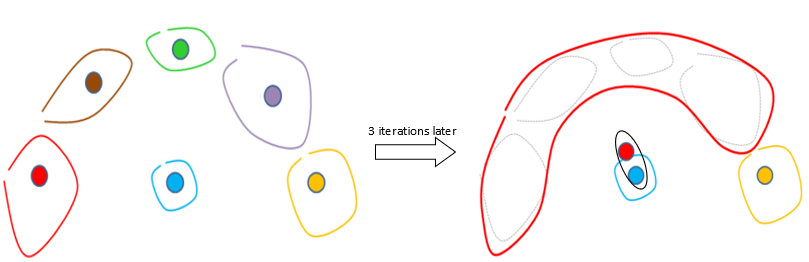
On the 4th iteration of the standard Ward’s algorithm, the red segment will be erroneously aggregated with the blue segment (instead of the yellow segment) (because the center of the red segment is closer to the center of the blue segment than the center of the yellow segment). The problem comes from the fact the segments are not spherical and thus the center of the red segment falls completely “outside” the red segment.
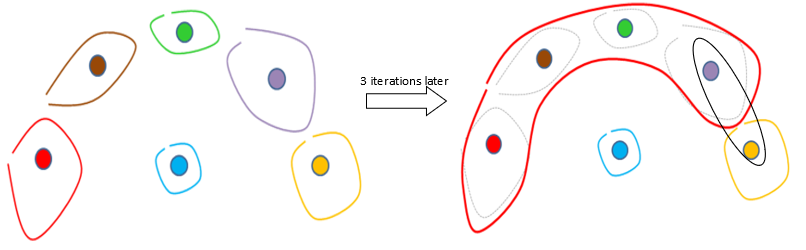
To correct this situation, we will use another algorithm named the “Minimum Spanning Tree” algorithm (or MST, in short). This new algorithm does not create “new centers” that could possibly be completely wrong (see the red center in the previous example): it only uses the “original” centers delivered by the K-means algorithm. It works this way:
1.Start with the segments found by the K-Means algorithm. Create one “Meta-segment” for each original segment.
2.Search for the two closest segments ![]() and
and ![]() amongst all the original segments delivered by the K-Means algorithm. Do NOT include inside the search all the pairs (
amongst all the original segments delivered by the K-Means algorithm. Do NOT include inside the search all the pairs (![]() ,
,![]() ) where
) where ![]() and
and ![]() belongs to the same “meta-segment”.
belongs to the same “meta-segment”.
3.Mark the segments ![]() and
and ![]() as belonging to the same “meta-segment”
as belonging to the same “meta-segment” ![]() that is the sum of the “meta-segment” including
that is the sum of the “meta-segment” including ![]() and the “meta-segment” including
and the “meta-segment” including ![]() .
.
4.If there is only one “meta-segment” then stop, otherwise go back to point 2.
Thus, at each iteration of the MST algorithm, the number of meta-segment is decreased by one. We can now easily select how many meta-segments we want by selecting how many iteration of the MST algorithm we will do. The “meta-segments” of the MST algorithm are equivalent to the “segments” of the ward’s algorithm.
The MST algorithm is working fine on the previous difficult example because at the 4th iteration of the MST algorithm the red segment will be correctly aggregated with the yellow segment.
TIMi is the only segmentation/datamining tool that offers you the MST algorithm that allows you to define “non-spherical” segments.
Both the standard Ward’s algorithm and the MST algorithm are computing distances between segments. We have already talked a lot about distances between points/individuals of our dataset (see section 5.5.1) but not between segments. There are two different “distances between segments” available inside StarDust:
1.Generalized distance: 
2.Simple distance: ![]()
... where ![]() is the segment A.
is the segment A.
![]() is the sum of all the row-weight of the individuals belonging to segment A.
is the sum of all the row-weight of the individuals belonging to segment A.
![]() is the center of the segment A.
is the center of the segment A.
![]() is the distance between the points A and B as defined in section 5.5.1
is the distance between the points A and B as defined in section 5.5.1
The Generalized distance has the tendancy to create equal-size segments.
The Simple distance creates segments of any size.
To summarize, we have:
|
Simple distance (allow discovery of small segments) |
Generalized Distance (produces equal-size segments) |
standard Ward’s algorithm (spherical segment) |
Classical Ward (option 1) |
Generalized Ward (option 3) |
Minimum spanning tree (MST) algorithm (non-spherical segments) |
MST- Minimum spanning tree (option 2) |
Generalized MST- Minimum spanning tree (option 4) |
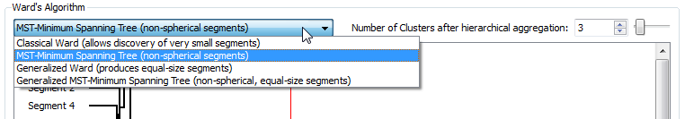
These 4 different options are available here: