For your first lecture of this guide, I suggest you to skip this section a go directly to section 5. In this section, we will assume that you are familiar with the usage of StarDust.
Inside StarDust, all the algorithms (PCA, K-means & Ward) are able to take into account user-defined “weights” on the columns and on the rows.
A large weight on a row of your dataset means that this particular individual is very important. A large weight on a column of your dataset means that this column is very important. You can set the row-weights here: ![]() and the column-weights here:
and the column-weights here: ![]() .
.
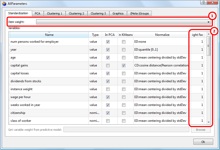
The column-weights are designated as ![]() in section 5.5.1.
in section 5.5.1.
The sum of the row-weights inside a segment is designated as ![]() in section 5.5.3.2.
in section 5.5.3.2.
There exist some optimal column-weights that allow you to visualize in an optimal way the characteristics that separate your “Target Group” from the rest of the population. When you are using these optimal column-weights, you can easily “see” and “explore” your “Target Group” in relation to the other individuals.
For example, for the census-income database:
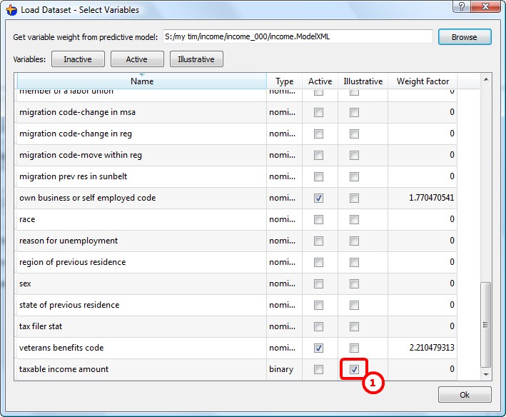
Note that we added as illustrative variable the “taxable income amount”. ![]()
A good idea is to also add as illustrative variable the “sex”.
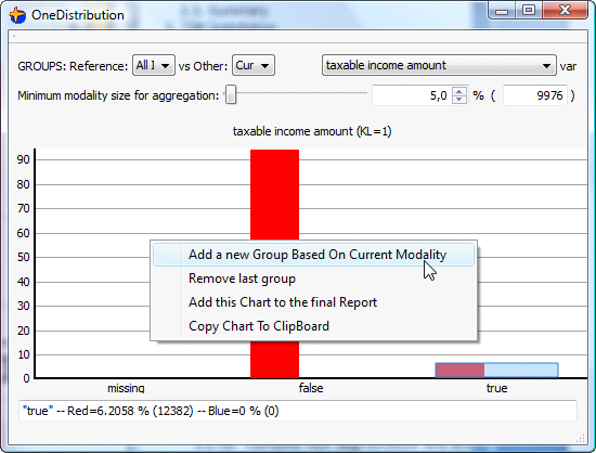
Thereafter, we load the dataset. We go directly to the chart representing the variable “Taxable income amount” (click The ![]() button) and we add the “True” modality as a new group.
button) and we add the “True” modality as a new group.
Let’s configure the display of our Groups: click the ![]() button and select the “(Meta-)Group” tab:
button and select the “(Meta-)Group” tab:
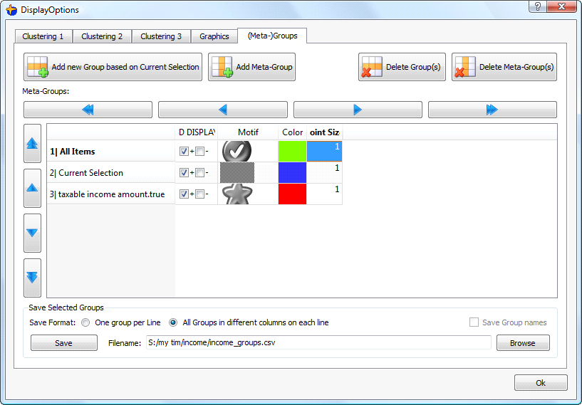
... and we finally obtain:
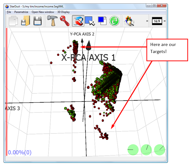
Apparently, in this case, the “Target Group” is roughly divided in two parts! This is interesting... We should investigate what’s the difference between these parts.