After clicking the ![]() icon, you switched to “Expert” mode. While in “Expert” mode, you can:
icon, you switched to “Expert” mode. While in “Expert” mode, you can:
•Add new parameters (and edit the parameters) of the Action: ![]()
•See the other panels of the R box: ![]()
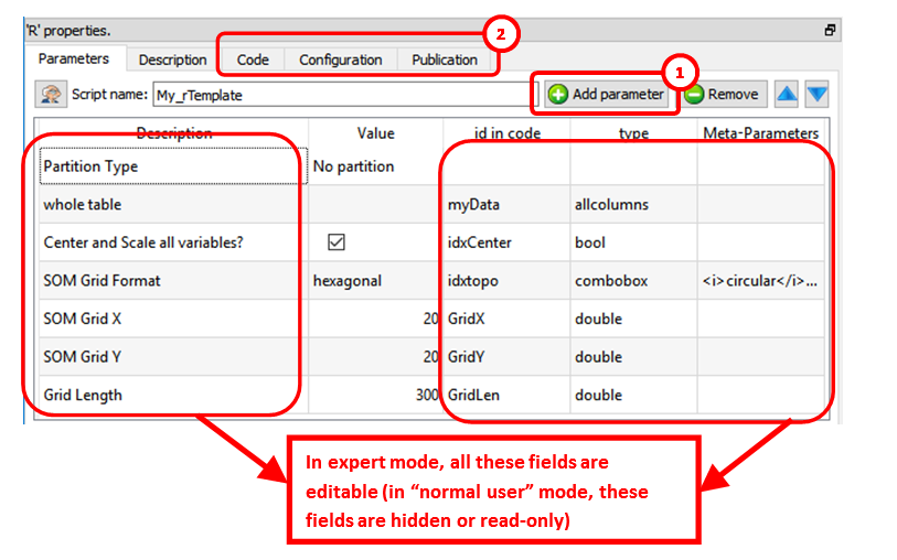
In the above example, we can see that Anatella will initialize the R engine with 6 variables (these 6 variables are named “myData”, “idxCenter”, “idxtop”, “GridX”, “GridY, “GridLen”) before running the R code. All the parameters that are tables (coming for the input pins) are injected inside the R engine as “data frames”.
In particular, the “Code” panel is interesting: it contains the R code: Here is an example of R code:
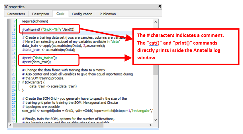
You can use the "print()" or the “cat()” command to display some values inside the Anatella Log window (this is useful for debugging your code).
![]()
When the R engine prints some results inside the Anatella Log Window, it assumes that the font used to display the results is of Constant-Width (e.g. so that, we you print an array, the different columns from your array are correctly aligned on each row).
By default, Anatella uses a Variable-Width font inside the Log Window (and thus the array’s are not displayed very nicely).
You can change the font used inside the Log Window here:
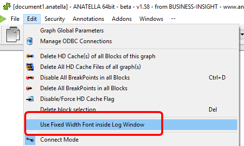
(You can also use “CTRL+Wheel” to zoom in/out the text inside the Log Window)
![]()
The # characters at the start of a line indicates a comment. Inside R, there are no easy way to comment several lines of codes (i.e. there are no /*…*/ as in other languages such as Javascript, C, C#, Java, etc.).
Here is a special extension that is only available inside Anatella: Use the string “##astop” (without the double-quotes at the beginning and the end) at the very start of a line to prevent Anatella to execute any R code located beyond the “##astop” flag. This is handy when developing new R Actions.
Here are some “good practice” rules to follow when creating a new R code:
1.It might be easier to use an interactive tool such as “R-Studio” to develop the first version of your R code (i.e. during the first “iterations” of code development). Once your R code is working more-or-less properly, you can fine-tune its integration inside an Anatella box using the Anatella GUI. Once the integration inside Anatella is complete, you’ll have a block of R code (i.e. an Anatella box) that you can re-use easily everywhere with just a simple drag&drop! (…and without even looking at the R code anymore!)
![]()
When developing a new code in R, it happens very often that the R engine computes for a very long time (for example, because you didn’t define properly a parameter) and the whole data-transformation is “freezing” abnormally for very long period of time. In such situation, don’t hesitate to click the ![]() button inside the toolbar to abort all the computations prematurely. The Anatella GUI remains stable even if you cancel all the time the R engine. This allows to make many iterations, to quickly arrive to a working code.
button inside the toolbar to abort all the computations prematurely. The Anatella GUI remains stable even if you cancel all the time the R engine. This allows to make many iterations, to quickly arrive to a working code.
2.If you need a specific data-type to run your R computations, ensure that you convert to this specific data-type before doing any computation. For example, don’t assume that you’ll always receive a matrix full of numbers in input: More precisely: Always force the conversion to the “number type”, if you specifically need “numbers” to do your computations. To convert a data frame (received as input) that is named “myDataFrame” into an Array of numbers (and get rid of the strings!) that is named “myArray”:
myArray <- apply (as.matrix (myDataFrame), 2, as.numeric);
3.If you need some specific packages in order to run your R code, add a few lines of code (at the top of your R script) that installs the required packages if they are not there yet. For example, this install the “kohonen” package if it’s not there yet:
if("kohonen" %in% rownames(installed.packages()) == FALSE)
{
print("installing cohonen package for first time use");
install.packages("kohonen",repos=RemoteRepository)
}
(don’t forget to use the option “repos=RemoteRepository” inside the above “install.packages” command)
When creating a R box that displays some plot window:
1.in the “Configuration” panel, check the option "This Action creates some plot windows" (otherwise the “plots windows” are destroyed as soon as the box stops running):
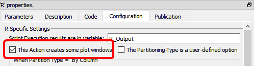
2.Use "x11();" to open new “plot windows” (otherwise all plots ends up inside the same plot-window and you only see the last plot because it has “overwritten” all the previous ones)
3.Optional: To avoid consuming much RAM memory for nothing (while R is just busy showing your plots), add at the end of your R code a few lines to destroy all large matrices stored in RAM. For example:
#free up memory:
myDataFrame=0; # replace the large data-frame named “myDataFrame” with
# a single number (0) to reclaim RAM
gc(); # run garbage collector to force R to release RAM
To pass back some table-results as output of the R Action, use the “R_Output” variable. The data-type of the variable used as output is very precise: it must be a data frame (and not an array). To convert your variables to data frames, use the following command:
myDataFrame <- data.frame( MyVariable, stringsAsFactors=FALSE)
(don’t forget the option “stringsAsFactors=FALSE”, otherwise R does strange things!!).
Here are some example of usage of the output variable named “R_Output”:
1.To pass on output pin 0 the data frame named “myDataFrame”, simply write:
R_Output <- myDataFrame
Please ensure that the type of the variable named “myDataFrame” is indeed a “data frame” (and not an “Array”), otherwise it won’t work.
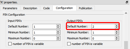
2.To pass on output pin 0 the data frame named “myDataFrame1” and to pass on output pin 1 the data frame named “myDataFrame2”, simply write:
R_Output <- list(myDataFrame1, myDataFrame2)
For the above code to work, you must also setup Anatella to have 2 output pins on your box:
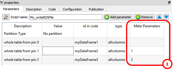
To get inside the R environment the input tables available on the second, third, fourth,... pins, use the column “Meta–Parameters” inside the “Parameters” panel: ![]() For example, this define 3 data frames (named “myDataFrame1”, “myDataFrame2” and “myDataFrame3”) that contains the tables on the input pins 0,1 & 2:
For example, this define 3 data frames (named “myDataFrame1”, “myDataFrame2” and “myDataFrame3”) that contains the tables on the input pins 0,1 & 2:
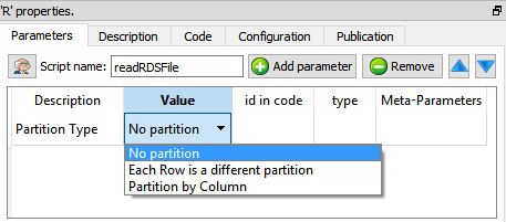
The R engine is quite limited in terms of the size of the data it can analyze because all the data must fit into the (small) RAM memory of the computer. To alleviate this limitation of R, you can ask to Anatella to partition your data. There are currently 3 different partitioning options inside Anatella:
How does it work? The table on the first input pin (i.e. on pin 0) is “splitted” in many different “little” tables (the tables on the other pins – pin 1, pin 2, pin 3, etc. – are always injected completely inside the R engine without any “splitting”). The R engine can process easily each of this “little” table because they only consume a small quantity of RAM memory. After the split, Anatella calls the R engine “in-a-loop”, several times: At each iteration, the R engine process one different “little” table (and it might also produce some output).
There are three “Partition Types”:
•No partition (the default option): self-explaining.
•Each Partition has the same number of rows (with the exception of the last partition): self-explaining.
•Partition by Column: When using this option you must select a “Partitioning Column”. For example, if you select as “Partitioning Column” the column “Age”, then each partition will containing all the people (i.e. all the rows) with the same “Age”.
The concept of “Partition” is used many times inside Anatella: e.g. See the sections 5.5.3. (Partitioned Sort), 5.17.4 (Time Travel), 5.7.9. (Quantile), 5.5.9. (Flatten), 5.3.2.5. (Multithread Run), 5.17.2. (Smoothen Rows) of the “AnatellaQuickGuide.pdf” where the same partitioning concept is also used.
More precisely, when using partitioning, Anatella does the following:
1.Split the table on pin 0 into many different “little” tables
(one table for each different partition).
2.Inject into R the variables that contains that data from all the rows of the tables available on pin 1, pin 2, pin 3, etc.
3.Inject into R the variable named “partitionType” (whose value is 0, 1 or 2, depending on which “Partition Type” you are using).
4.Inject into R the variable named “iterationCount” with the value 0.
5.Inject into R the variable named “finished” with the value “false”.
6.Run the loop (i.e. process each partition):
oInject into R one of the “little” tables (that are coming from the “big” table available on the first input pin – input pin 0).
oRun your R code inside the R engine.
oGet back some output results to forward onto the output pin.
oIncrease by one the value of the R variable “iterationCount”.
oExecute the next iteration of the loop (i.e. re-start step 6) until there are no more “little” tables to process.
7.If the Anatella option “Execute one "Final" iteration with a NILL input when executing with a partition” is checked (i.e. it’s TRUE):
oSet the variable named “finished” to the value “true”.
oReset the variables that contains the “little” tables to NILL
oRun the R engine one last time.
oGet back some output results to forward onto the output pin.
![]()
One example where partitioning “makes sense” is when you want to use a predictive model to score a new dataset. In opposition to “learning datasets”, “scoring datasets” can be really big (so big that they don’t fit into RAM). When you use a partition, you can compute the predictions for any (scoring) dataset, whatever the size of the dataset. Nice! J
![]()
Another example where partitioning “makes sense” is the following: Let’s assume that you are working for a large retailer (such as Carrefour, Wallmart, etc) and you need to manage the stocks of all your different products (the products are also named “SKU”=Stock Keeping Unit) at all your different Point-Of-Sales (POS). One important part of stock management involves predicting what will be the demand of each (SKU;POS) pair in the forecoming weeks. If you predict a high demand for a specific (SKU;POS) pair, then you’d better have a significant stock for this same (SKU;POS) pair (unless you want to lose sales because of “out-of-stock” conditions). A typical large retailer has around 20,000 SKU’s at each of their POS. Let’s assume that we have 200 POS. We thus have 20,000x200=4,000,000 (SKU;POS) pairs. This means that we’ll have to compute 4,000,000 predictions (one for each (SKU;POS) pair). This also means that we’ll typically have a matrix with 4,000,000 rows: Each row contains information about the past demand for a (SKU;POS) pair. Using the values available on the current row (about past demands), we’ll typically use some “time series” algorithm to predict the future demand (for the forecoming weeks). Actually, to compute the prediction for a specific (SKU;POS) pair, you only need one row of the table. In other words, all computation can be done row-by-row. This means that we can use the “Partition Type” named “Each Row is a different partition”. Because of the Anatella-Partitioning-Algorithm, we can handle any number of SKU or POS without being limited by the R engine when it comes to handle large matrices.
There is also a “Kill R” button inside the toolbar here:
This button kills all the R engines currently running. This means that, when you click this button:
•All (R-based) plot-windows are closed
•All R computations are stopped (i.e. don’t click this button when your graph is running!).
![]()
TIP: Use the ![]() button inside the toolbar to close in one click all the plot-windows.
button inside the toolbar to close in one click all the plot-windows.
Once you are satisfied with your R-based Action, you can “publish it” so that it always becomes available inside the “common” re-usable Actions: See section 9.7. for more details on this subject.