<< Click to Display Table of Contents >> Navigation:  5. Detailed description of the Actions > 5.16. TA - Operational Research > 5.16.1. Assignment Solver (High-Speed action)

 

Icon:

 
Function: AssignmentSolver
 

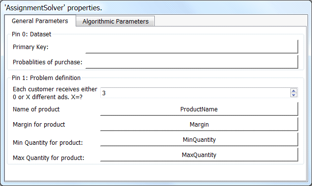
Property window:

 

 

 

 

 

 

Short description:

 

Solve the constrained assignement problem.

 

Long Description:
 

The constrained assignment problem is a very classical problem that occurs very often in direct marketing. It’s also very common in retail. The typical usage is the following:
 

•The setting: You have a limited number of “promotional coupons” for 100 different products. Each of these coupons is offering a reduction on a specific product. Each of these coupons is in limited quantity because they are given by the corresponding product supplier in limited quantity. You can think about these 100 products as the “highlighted products of the week”.
 

•The objective: Use the promotional coupons to attract some customers into your store to have the opportunity to sell them some more products.
 

•How? Each of your customers will receive 5 coupons (out of a total number of 100 different coupons associated to 100 different products). To redeem the coupons your customer need to come into your store. We’ll select the 5 coupons that are the “most-likely to be redeemed”. These 5 coupons are different for each customer. These 5 coupons are selected using predictive modeling:

Each of the coupons corresponds to a specific product. We’ll build 100 predictive models that compute the probability of purchase for each of the 100 products. We then “apply” these 100 models to get, for each cutomers, 100 purchase probabilities. In the simple case (when there are no constraints), the 5 coupons (that a specific customer receives) correspond to the top-5 probabilities out of the 100 probabilities that are computed for each customer (using our 100 predictive models).
 

•The difficulty: There are constraints: You cannot simply assign to a customer the products with the highest purchase-probabilities (and totally disregard the limitation on the quantity of each product). When such a constraint (on the quantity of each product) exists, the assignment of a specific product to a specific customer must be computed using a more complex mechanism: This is the objective of the AssignmentSolver Action.

 

 
The classical methodology used to optimally assign coupons to your customers is:
 

•For each different product (or "coupon"), create one predictive model.

•Apply all the predictive models on the customer database to obtain, "For each customer, the probablity of purchase of each product".

•Assign coupons to each customers so that:

oThe Expect Return (ER=ROI) of the campaign is maximized

 (i.e. The customers are receiving the coupons related to the products that they are the most likely to buy).

oThe constrained are respected: These are:

▪The amount of coupons of each product is limited to a given threshold.

▪Each customer receives exactly n coupons.

(i.e. one folder contains exactly n coupons for n different products).

 

This procedure assigns a different set of products (or “coupons”) to each customer. Potentially, there are as many different folders as there are customers (To print these folders you need a “digital printer” because this is the only technology that allows you to print a different folder for each customer).

 

There exist two types of assignment problems:

 

1.Mono-product assignment problems: You need to select ONE product per customer, taking into account the constraints.

 

These type of problems can easily be solved with any number of highlighted products and any number of customers: For example:

 

For each different customer, propose 1 product amongst 9 different products.

 

The Mono-product solver uses the concept of "meta-customer". A "meta-customer" is a mini-segment of customers computed using Stardust. Typically, we’ll have 300 to 1500 differents segments. This type of assignment problem is easily solved using any LP solver (Anatella has a very high-quality multi-threaded LP solver).

 

2.Multi-product assignment problems: You need to select n>1 products per customer, taking into account the constraints (n is the number of coupons inside a folder).

 

These type of problems are extremely difficult to solve because they belong to the class of problem known as "NP-hard" problems. For example:

For each different customer, propose 3 products amongst 9 different products.

For each different customer, propose 8 products amongst 450 different products.

Because these problems are “NP-hard”, it’s not possible to solve them exactly. The AssignmentSolver Action uses advanced meta-heuristics to find a “good-enough” solution in a reasonable amount of time.

 

 

About “NP-Hard” problems.

Typically, to solve a “normal” numerical problem (i.e. not a NP-hard problem), a good idea is to “split” the problem into simpler problems, then solve each simpler problem separately and thereafter combine all these intermediate results into the “final” solution.

 

This type of approach is not possible with “NP-Hard” problems: They are not decomposable. The only way to exactly solve “NP-Hard” problems is to enumerate all possible solutions and to give, as the “final” solution, the best admissible solution found during the enumeration.

 

Let’s now evaluate how much time is required to enumerate all possible solutions to the multi-product assignment problem. Let’s assume that, inside our assignment problem, there are c customers and p products. One solution of the assignment problem is a matrix X. Each element Xij of the solution-matrix X is, either:

“Xij=1”: the customer i             received a coupon about product j.

“Xij=0”: the customer i did not receive   a coupon about product j.

We need to enumerate all the different solution-matrices X.

There are 2c x p different solution-matrices X.

For a normal-size problem, we have: c=1 million customers, p=100 products, the number of different solutions: 2100 million= a very very large number.

Even on the best possible hardware, it will take several times the age of the universe to enumerate all the solutions.

 

 

Since it’s not possible to solve exactly the multi-product assignement problem (because it’s not possible to enumerate all different solutions), we’ll only try to find a “good enough” solution: We’ll enumerate only a (very) limited number of good “candidate solutions”. These “candidate solutions” are generated using a meta-heuristic named “tabu-search”. The solution that is returned by the AssignmentSolver Action is the best admissible solution found during this “limited” enumeration.

 

 

“Admissible solution” means a solution that respects the constraints (i.e. The constraints are: We have some limitations on the quantity of each coupon/product).

“Best solution” means a solution that has the highest ROI/the highest ER.

 

 
The quality of the returned solution mainly depends on the running time: If you run the “tabu-search” procedure for a very-long time, you’ll be able to test a large number of different “candidate solutions” and you’ll be more likely to find a very good solution (To summarize: the longer you compute, the better the “returned” solution).

 

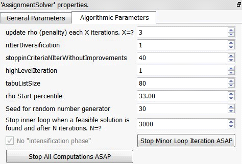
The different parameters of the AssignmentSolver Action control are:

1.the running-time (i.e. these are parameters used as “stopping criterias”)

2.the way the “candidate solutions” are generated using the “tabu-search” procedure.

 

The solution returned by the AssignmentSolver Action is a table that contains the primary keys of each customers and the solution-matrix X. Each element Xij of the solution-matrix X is, either:

“Xij=1”: the customer i               received a coupon about product j.

“Xij=0”: the customer i did not receive   a coupon about product j.

 

More precisely, inside the solution table, we have:

1.Each row is a customer.

2.The columns are:

oThe primary key of the customer.

oThe different products assigned to the customer: These are p different columns (p=number of highlighted products) that contains either “0” (i.e. the product is not assigned to this customer) or “1” (i.e. the product is assigned to the current customer).

 

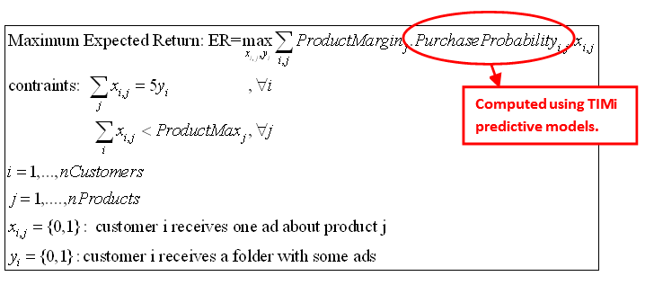
In mathematical terms, the best solution is the solution that cumulates the greatest purchase probabilities for all the assigned products to all the customers: It’s:

Best solution is the one that solves:

 

With   i=1,…,c  : all the customers  (there are c different customers in total)

j=1,…,p  : all the “highlighted products of the week” (there are p different highlighted products in total).: this is typically computed using 100 predictive models (one model for each different highlighted product).

 

 
Furthermore, this solution must respect these 2 constraints:
 

1.The number of coupons per product is limited (this is a user-specified business constraint):

2.Each customer receives 5 ads (this is thus a multi-product assignment problem and not a mono-product assignment problem because 5>1)(one folder contains 5 coupons):

Let’s now assume that you get a small margin each time a customer uses a coupon. The “expected profit” when a customer i purchases a product j is thus:

 

The table returned by the AssignmentSolver Action is the solution Xij to the following optimization problem:

 

To use the AssignmentSolver Action, you need to provide these 2 input tables:
 

1.Probability Table: On input pin 0: one row= one customer: This table contains:
 

oThe primary key of each customer

oThe for all customers and all products. These probabilities are typically computed using TIMi.
 

2.Problem-DefinitionTable: On input pin 1: one row=one highlighted product: This table contains 3 columns:
 

oThe name of the product: This name must match the corresponding column name inside the Probability Table.

oThe (margin on each of the product)

oThe (the constraint: i.e. the maximum available quantity of coupons related to this product)

 
 

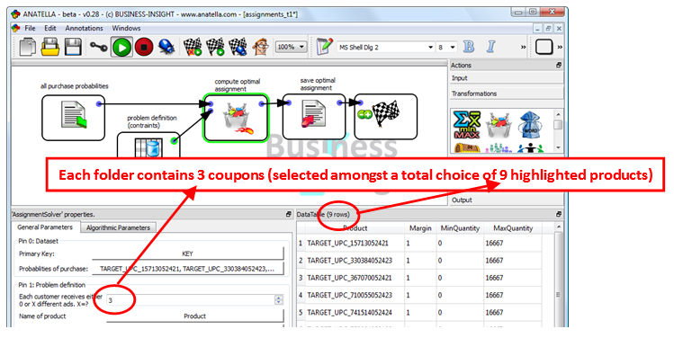
Here is an example:

 

 

The AssignmentSolver Action uses a “tabu-search” procedure to generate many good “candidates solutions”. At the end, we’ll return the best, admissible candidate solution (i.e.: The one with the highest ER=“Expected Return” that satisfies all the contraints). The “tabu-search” procedure is an iterative procedure: it starts from a known candidate-solution and “changes” it slightly to create a new candidate solution. For example, this small “change” can be: Swapping 2 products between 2 different customers. The “tabu-search” procedure always tries to make a change that improves the “quality of the candidate solution”. To avoid entering inside the “infeasible space” (i.e. to avoid entering the space composed of solutions that do not satify the constraints), the “quality of the candidate solution” is defined as:
 

 
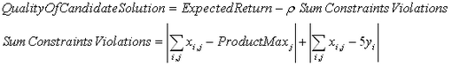
If the parameter is very small, the “tabu-search” procedure will allow “entering” the infeasible space.

If the parameter is very large, the “tabu-search” procedure will be “pushed” towards the feasible space.

 

If there are many violated contraints inside the current solution, the assignement solver automatically increases the parameter to “go back” towards the feasible space. Allowing the assignement solver to enter slightly inside the infeasible space is an important feature to avoid getting stuck “inside a local optimum” along the way toward the “best” solution.

 

It can happen that the next best candidate solution is a solution that we already tested previously. This is annoying because it can cause “infinite loops” inside the assignement solver (e.g. the solver always “circle around” testing always the same set of candidate solutions). To avoid such phenomenon, the solver keeps a list of “tabu” solutions (thus the name: “tabu-search”). A candidate solution is marked as “tabu” when it has been already “explored” at a previous iteration of the solver. The solver is then forbidden to “move to” a “tabu” solution. The “tabu-list” of forbidden solutions prevents the solver to “circle around”. The tabu-list is also a very effective mechanism to “get out” of local optimum (to be able to find the “global” optimum).

 

The size of the “tabu-list” is limited using a FIFO methodology (FIFO=first in, first out). A large tabu-list allows you to be less sensitive to local optimums (and this is good) but it also increases significantly the running time.

 

The quality of the solution depends on the quality of the candidates generated by the tabu-search algorithm. To generate these candidates, at each iteration of the “tabu-search” procedure, we apply a small “change” to the current solution. These “incremental changes” must have several properties:
 

1.It should be easy (i.e. fast) to compute if a change has a positive or a negative impact on the “quality of the solution”.

2.These changes should allow you to avoid getting “stuck” on sub-optimal solutions. More precisely: They should allow you to quickly explore *all* the different part of the feasible space (and not a small, limited part of the feasible space). This means that these “changes” must be very varied in nature.

 

Unfortunatly the 2 properties hereabove are antagonist objectives. More precisely: you can have:
 

1.“simple” changes: These are quick to compute but they do NOT “cover” correctly the complete feasible space (and thus you might miss the optimal, best solution using only these “simple changes”).

2.“complex” changes: These are slow to compute but that allow you to explore “in-depth” all the feasible space.

Here are the differents steps that are executed inside the multiproduct assignement solver to compute the (near) optimal assignement:
 

1.STEP 1. Generate a first “candidate solution” using very simple heuristics. The quality of this very first solution is very weak (i.e. The ER is very low). The algorithms used in this phase are very simple and could be implemented in nearly any scripting language (including SAS).

2.STEP2. Fast solver:

a)Use a very fast “tabu-search” procedure that only involves “simple changes” to quickly improve the solution found at the previous step. The “tabu-search” procedure is allowed to enter inside the infeasible space (the parameter is small)

b)Use a simple heuristic to find the closest feasible solution to the solution found in step 2.a).

c)Use a very fast “tabu-search” procedure that only involves “simple changes” to quickly improve the solution found at step 2.b). The “tabu-search” procedure is *NOT* allowed to enter inside the infeasible space.

3.STEP 3. In-depth solver:

a)Use a slow “tabu-search” procedure that involves “complex changes”. Dynamically adjust the parameter to allow to temporarily enter inside the infeasible space. If the ExpectedReturn (ER) of the solution does not improve for a large number of iterations, we break and go to step 3.b).

b)The solution produced at step 3.a) is the best solution that we can obtain using:

1.The (limited) set of “complex changes” that are implemented inside the assignment solver.

2.A given starting point

Let’s scramble the current best solution using a large number of completely random perturbations. We now have a low-quality (and possibly infeasible) solution. Go back to step 3.a) and use this low-quality solution as starting point for the “tabu-search” procedure. This new starting point might (maybe) allow us to reach a better solution.

 

The “tabu-search” algorithms used during the steps 2&3 are carefully tuned C++ implementation. The extremely high speed of the C++ solver included inside Anatella allows us to explore a larger number of different candidate solutions than any other implementation, leading to a better solution (more ROI) at the end.

 

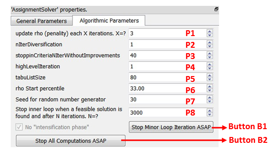
The parameters that control the solver are:

 

 

As usual with all meta-heuristics, the more time we explore the search space, the better the quality of the final, returned solution. Thus, it’s important to avoid losing time exploring un-interesting regions of the search space.

 

1.Parameter P1: “Update rho each X iterations. X=?”.

During step 3.a), the parameter is dynamically adjusted every X iterations.

1.1.If the parameter P1 is too large we can inadvertently enter “deeply” inside the infeasible space. We’ll then lose time simply “moving back to” (i.e. restoring) feasibility.

1.2.If the parameter P1 is too small, we can get “stuck” in a local optimum and find a really poor solution.

 

2.Parameter P2: “nIterDiversivication”

During step 3.b), we scramble the best know solution to obtain a new starting point for further optimization. The parameter P2 controls the amount of “scrambling” that is applied.

2.1.Too little “scrambling” and we’ll re-explore again the same set of solutions that we already explored (and thus we won’t find a better solution).

2.2.Too strong “scrambling” and we’ll move really far away from the “region of interest” (i.e. the region of the search space that is the most likely to contain the optimal solution). We’ll then lose a large amount of computing time just to “go back” to the “region of interest” (and this computing-time could be used more efficiently searching inside “region of interest” for the best solution).
 

3.Parameter P3: “stoppingCriteriaNIterWithoutImprovements”

During step 3.a), we’ll run a slow “tabu-search” procedure that stops when the ExpectedReturn (ER) of the solution does not improve for P3 iterations.

3.1.If the parameter P3 is too small, we can abort prematurely the “tabu-search” procedure and potentially “miss” a very good solution.

3.2.The final solution found by one run of the “tabu-search” procedure (in step 3.a)) depends on the “starting point” (i.e. the candidate-solution that was used to initialize the “tabu-search” procedure). Some “starting points” generate better final solution than others. The objective of the “high-level” loop (that is composed of steps 3.a) and 3.b)) is to “test” different “starting points” (to see which one generates the best solution at the end). If the parameter P3 is too large, we might lose time investigating the outcome of an uninteresting “starting point” (Maybe it’s better to “investigate” very roughly many different starting points than to “investigate” very deeply the outcome of a small number of starting points).

 

4.Parameter P4: “highLevelIteration”

The parameter P4 is the number of iterations inside the “high-level” loop (that is composed of steps 3.a) and 3.b)). The objective of this “high-level” loop is to “test” different “starting points”.

If the parameter P4 is zero, then only the “fast solver” is used.

Proceed with caution when increasing P4: This increases a lot the running time of the multiproduct assignement solver.

 

5.Parameter P5: “tabu-list size”

A large tabu-list allows you to be less sensitive to local optimums (and this is good) but it also increases significantly the running time.

 

6.Parameter P6: “rho start percentile”

The parameter P6 controls the initial value of the parameter inside the (slow) “tabu-search” procedure that runs in step 3.a).

6.1.If the parameter P6 is too small we’ll start the tabu-search from a candidate-solution that is “deeply” inside the infeasible space. We’ll then lose time simply “moving back to” (i.e. restoring) feasibility.

6.2.If the parameter P6 is too small, we can get “stuck” in a local optimum and find a really poor solution.

 

7.Parameter P7: “Seed for random number generator”

The “tabu-search” procedure (in steps 2.a) and 3.a)) has a strong random component.

The “diversification” procedure (in step 3.b)) has an even greater random component.

The parameter P7 defines the “seed” used inside the pseudo-random number generator that is used inside the multiproduct assignement solver. For more information about pseudo-random number generator, see:

http://en.wikipedia.org/wiki/Pseudorandom_number_generator

 

8.Parameter P8: “Stop inner loop when a feasible solution is found and after N iterations.N=?”

Ideally, the slow “tabu-search” procedure of step 3.a) uses the parameter P3 as the only stopping criteria. However, it can happen that the slow “tabu-search” procedure manages to continuously improve (i.e. at nearly each iteration) the ER of the “best found solution so far”. These improvements are totally negligible but they still prevent the stopping criteria based on parameter P3 to work properly. The parameter P8 is useful when such rare circumstance occurs. The parameter P8 places a hard upper bound on the maximum number of iterations performed inside the slow “tabu-search” procedure. The effects of a very small (or very large) value for the parameter P8 are the exact same effects as for the parameter P3.

 

The multiproduct assignement solver has also 2 buttons that are only active when the solver is running:
 

1.Button B1: “Stop minor loop iteration ASAP”

When you click the B1 button the loop inside the “tabu-search” in step 3.a) stops immediately. This is interesting when you notice (looking at the numbers inside log window) that the current “starting point” is not interesting: it won’t produce a better solution (i.e. a solution with a higher ER than the “best solution known so far”). In such situation, click the Button B1: the solver will directly “jump to” step 3.b).

 

2.Button B2: “Stop All Computations ASAP”.

The parameter P4 is the number of iterations inside the “high-level” loop (that is composed of steps 3.a) and 3.b)). If the parameter P4 is very high, the solver will run for a very, very long time (testing many different “starting points”). It can happen that you need the final assignement *now* (and you don’t want to wait for still another lengthy “high-level” iteration). In such situation, click the button B2: The multiproduct assignement solver will nearly instantaneously output the “best solution known so far”.

 

 
Large Assignment Problems

 
To solve large assignment problems, set to zero the parameter P4 (“highLevelIteration”):

 

This will only run the “fast solver” (and completely skip the “In-depth solver”). The “fast solver” has also a very small RAM memory consumption (especially compared to the RAM memory consumption of the “In-depth solver”). This allows you to solve really large assignment problems with a computer that has a very limited RAM memory.