Icon: ![]()
Function: JoinInput
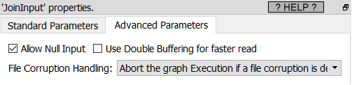
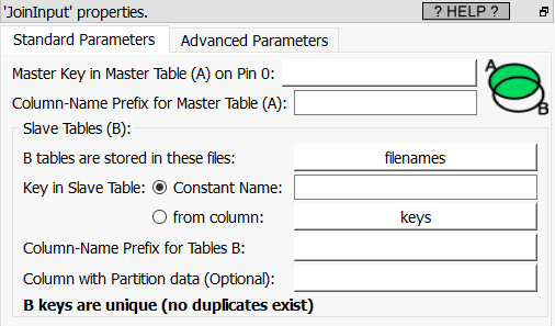
Property window:
Short description:
Left-Join several tables into one gigantic table.
Long description:
![]()
Pre-requisite
All the input tables must be sorted on the "Key" columns using the SAME sorting algorithm (all "numeric sort" or all "alpha-numeric sort").
The first step before creating any predictive model is to build a learning dataset that contains as many “good” features as possible (this is named “feature engineering”). Typically, each group of features is computed using one different Anatella graph. To gain time, you’ll usually run all the required “feature engineering” graphs in parallel (using the ![]() ParallelRun Action from section 5.3.3. or using the
ParallelRun Action from section 5.3.3. or using the ![]() loopAnatellaGraphAdv Action from section 5.20.6 or using the
loopAnatellaGraphAdv Action from section 5.20.6 or using the ![]() “Loop Jenkins” action from section 5.21.1). Each of these “feature engineering” graph delivers, as output, one small .gel_anatella file that contains some more features. The final step of the construction of your learning dataset is to “assemble” all these small .gel_anatella files into one large unique .gel_anatella file (that is your learning dataset). This “final assembly” might look like this:
“Loop Jenkins” action from section 5.21.1). Each of these “feature engineering” graph delivers, as output, one small .gel_anatella file that contains some more features. The final step of the construction of your learning dataset is to “assemble” all these small .gel_anatella files into one large unique .gel_anatella file (that is your learning dataset). This “final assembly” might look like this:
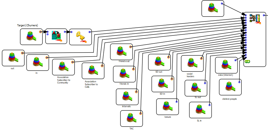
The above (real-life) example illustrates that, for a large number of different features, the construction of this “final assembly” might rapidly become an un-manageable graph with too many arrows and boxes (that looks like a plate of spaghetti! � ). At that point, you quickly understand why the ![]() JoinInput Action is really interesting!
JoinInput Action is really interesting!
To illustrate how to the ![]() JoinInput Action works, let’s look at a first example: The objective of this example is to add to a “customer.gel_anatella” table some additional features that are (initially) saved inside the 3 “slave” tables that are named “a.gel_anatella”, “b.gel_anatella” and “c.gel_anatella”. To make this assembly, we can use any of these two Anatella graphs:
JoinInput Action works, let’s look at a first example: The objective of this example is to add to a “customer.gel_anatella” table some additional features that are (initially) saved inside the 3 “slave” tables that are named “a.gel_anatella”, “b.gel_anatella” and “c.gel_anatella”. To make this assembly, we can use any of these two Anatella graphs:
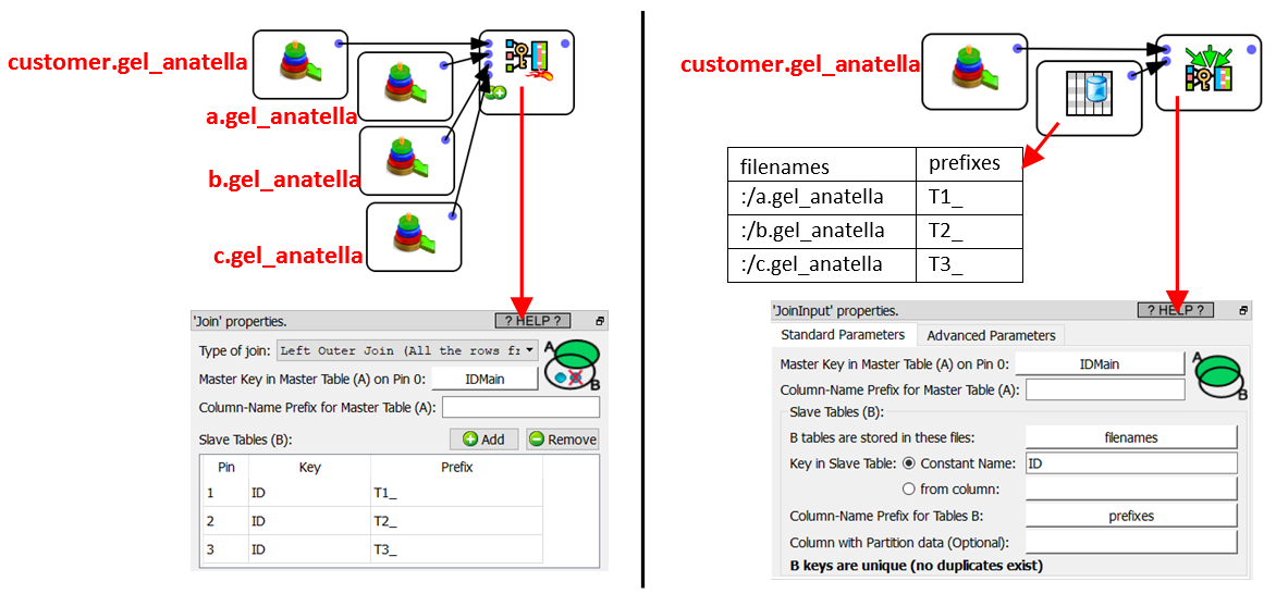
At first sight, these 2 graphs do look pretty similar in complexity. The main difference occurs when you increase the number of “slave” tables (that contains all the computed features) inside the Join (the above example only contains 3 “slave” tables: “a.gel_anatella”, “b.gel_anatella” and “c.gel_anatella”): With the ![]() JoinInput Action, you can easily have thousands of Slave tables, while the (other) approach based on the simple
JoinInput Action, you can easily have thousands of Slave tables, while the (other) approach based on the simple ![]() Join Action becomes un-manageable pretty quickly: Already with as little as 100 “Slave” tables, the Anatella graph is becoming a total mess to maintain&support: Just think about the number of boxes! (it will work but it will definitively be less manageable than the
Join Action becomes un-manageable pretty quickly: Already with as little as 100 “Slave” tables, the Anatella graph is becoming a total mess to maintain&support: Just think about the number of boxes! (it will work but it will definitively be less manageable than the ![]() JoinInput Action).
JoinInput Action).
![]()
The maximum number of “slave” tables inside the ![]() JoinInput Action is around 20000. This means that Anatella can effectively compute a Left join between 20000 tables! (as a comparison, the best databases are limited to 32 tables in a join)
JoinInput Action is around 20000. This means that Anatella can effectively compute a Left join between 20000 tables! (as a comparison, the best databases are limited to 32 tables in a join)
Let’s now assume that you need to create a learning/scoring dataset that has a very large number of rows. Each row represents one customer. To divide the computing time by 2, you decided to store the raw data collected on your customers on two different servers (the data from the customers with an odd primary key is stored on the first server and the data from the customers with an even primary key is stored on the second server). Then, when you are computing your features, you use both servers simultaneously (e.g. using the ![]() “Loop Jenkins” action from section 5.21.1). At the end of the feature computation, the first server contains all the features for half your customers and the second server contains all the features for the other half of your custromer. Then, you need to do the “final assembly”: To make this assembly, we can use any of these two Anatella graphs:
“Loop Jenkins” action from section 5.21.1). At the end of the feature computation, the first server contains all the features for half your customers and the second server contains all the features for the other half of your custromer. Then, you need to do the “final assembly”: To make this assembly, we can use any of these two Anatella graphs:
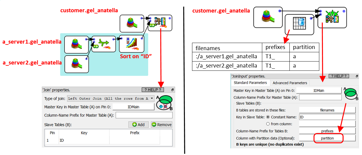
What happens if:
•…instead of using 2 servers, we use 3 servers?
•…instead of computing only the “a” features, we also compute the “b” and “c” feature sets?
To make the “final assembly”, we can use any of these two Anatella graphs:
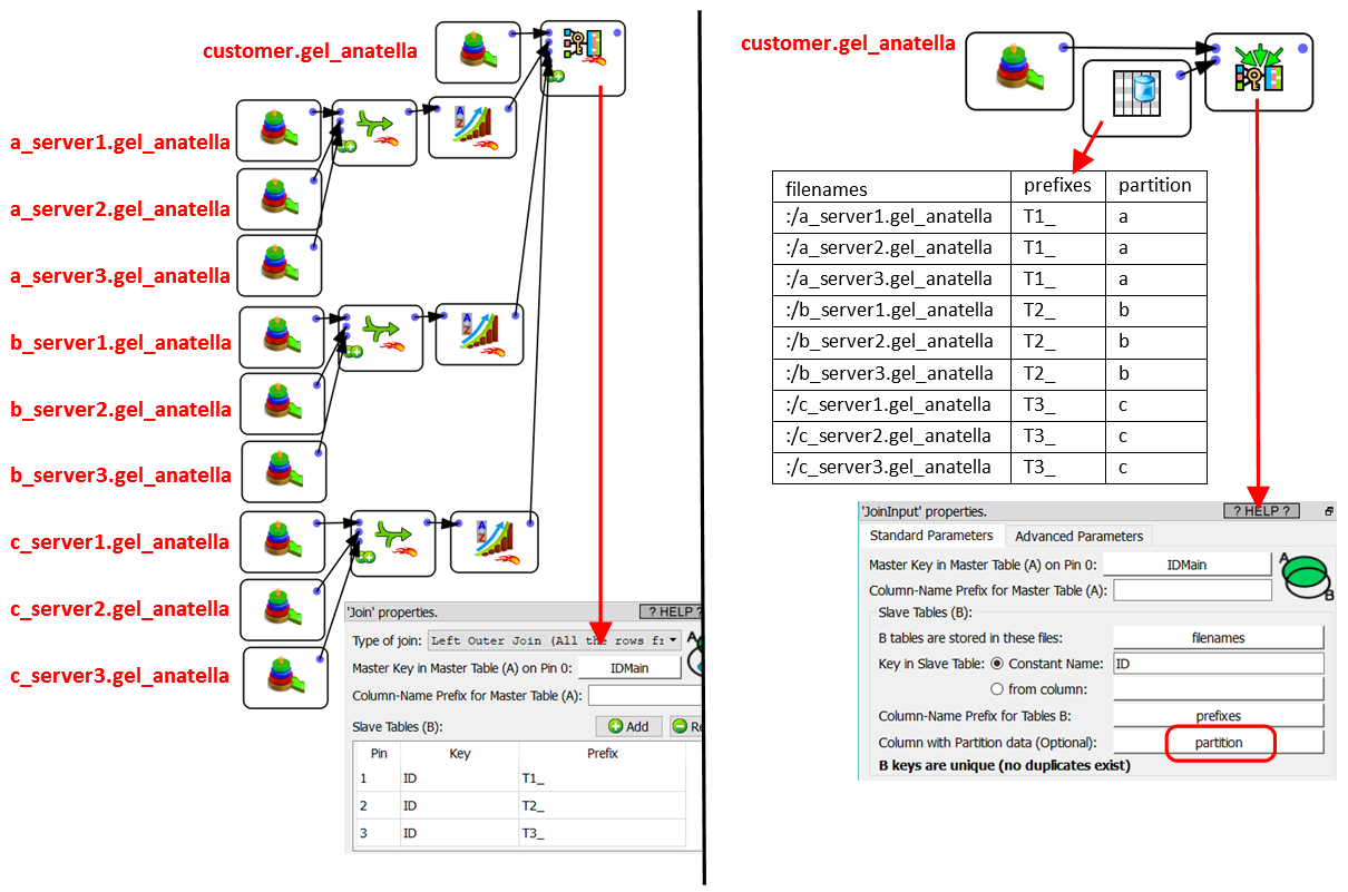
Inside the above example, all the partitions used for the ![]() JoinInput Action are composed of 3 files. In practice, each partition can have a different number of files: No worries!
JoinInput Action are composed of 3 files. In practice, each partition can have a different number of files: No worries! ![]()