<< Click to Display Table of Contents >> Navigation:  5. Detailed description of the Actions > 5.7. Data Mining > 5.7.1. TIMi Use Models (High-Speed action)

 

Icon:

 

Function: TIMiModelMerger

 

Property window:

 

 

 

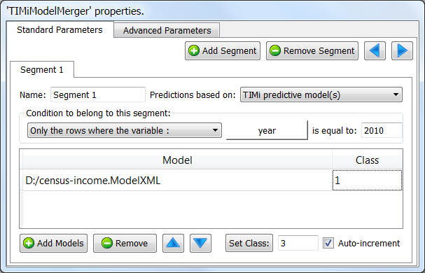
Short description:

 

Apply many TIMi predictive models on each row of the input table.

 

Long Description:

 

This operator applies many TIMi predictive models on each row of the input table.

 

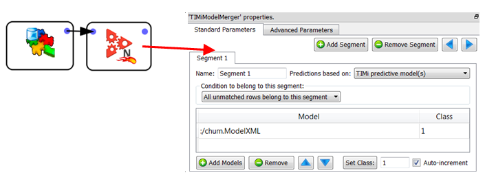
Let’s assume that we developed a simple churn model (i.e. we have a Binary Classification problem or, in other words, a scoring/ranking). We want to use this churn model inside Anatella. We’ll have:

 

 

Let’s now assume that you are developing a “next-to-buy” solution: i.e. You must guess which product out of these 5 products: TEDDY BEAR, LIGHT SABER, IPOD, FLOWER, BEER your customer will buy next. In the scientific world, this is known as a Multi-Class prediction system (in opposition to the classical Binary-Class prediction system: Did the customer churned or not? Yes/No).

 

To do multi-class prediction with TIMi, you must first transform the multi-class prediction problem into a series of binary classification tasks. These binary classifiers can be of one of the two types:
 

•1 vs all others
 

•1 vs 1

 
To know more about this subject, see section 6 of the “TIMi Advanced Guide”.

 

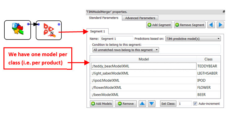
Let’s first investigate the simplest case: “1 vs all others”. In such a case, to make the prediction you need only 5 different binary predictive models (one for each product). You will apply these 5 models on each of the customers to obtain 5 purchase-probabilities (these 5 probabilities are different for all customers: This is true “one-to-one” marketing). The product with the highest purchase-probability will be the one that you will recommend as the next-to-buy. If you need to give a suggestion about 2 different products, you’ll take the 2 products with the 2 highest probabilities.

 

It can happen that the quantity of each different product is limited. In such a case, you cannot simply suggest the products with the highest purchase-probabilities (and totally disregard the limitation on the quantity of each product). When such a constraint (on the quantity of each product) exists, the assignment of a specific product to a specific customer must be computed using a more complex mechanism: see section 5.16.1 about the “assignmentSolver”.

 

Let’s return to a very simple case: More precisely:
 

•There are no constraints on the quantity of each of the products.
 

•We are using the “1 vs all others” type of predictive models.
 
We’ll have:

 

 

For the “1 vs 1” type of predictive models, we’ll have:

 

 

 

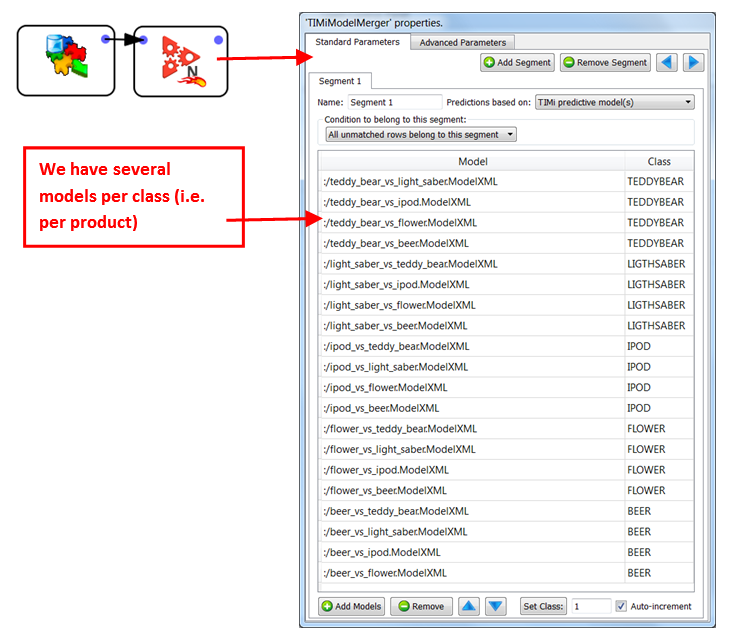
By default, when there are several models “voting” for the same class, the final (purchase) probability is the mean of the individual probabilities of each model. For example: The probability of buying a “teddy bear” is the mean of the 4 probabilities given by the 4 models:
 

•:/teddy_bear_vs_light_saber.ModelXML

•:/teddy_bear_vs_ipod.ModelXML

•:/teddy_bear_vs_flower.ModelXML

•:/teddy_bear_vs_beer.ModelXML

 
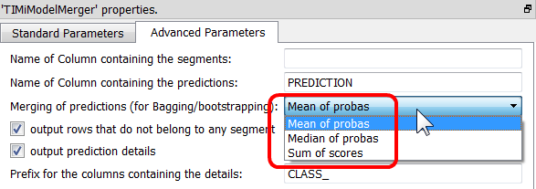
The “mean” operator is the default operator that is used to aggregate the individual probabilities of each predictive model to obtain the “final” probability for each different class (LIGHTSABER, IPOD, FLOWER, BEER). You can also use a different operator:

 

 

 

Even for simple Binary Classifier, it’s sometime interesting to use several predictive models (instead of just one). Depending on the way these models are created, this approach is either named “bagging”, “boosting” or “ensemble learning”. Why use several models instead of one? Because it usually delivers higher predictive accuracy.

 

 

Why do we get higher accuracy when using many models?

For example: Let's assume that we have 10 predictive models. The first 4 predictive models P1, P2, P3 & P4 always recognize and classify correctly the class C1 (they are “specialized” for C1). The other predictive models are specialized in other classes. Let's now assume that you want to classify a new example (i.e. a new row) and that this example belongs to the class C1. The 4 predictive models P1, P2, P3 &P4 will correctly answer C1. The other predictive models will give random answers that will form some "uniformly distributed noise" during the vote. The result of the vote will thus be C1. We just realized an error de-correlation.

How to generate the 10 different predictive models (BAGFS) ?

We don't have to know what’s the specialty of each of the predictive models. We only have to build predictive models that have various behaviors. We will build the 10 different predictive models using 10 different learning datasets. How do we generate these 10 learning datasets? We will use only a small part (called a bootstrap) of the “full” learning dataset (this technique is called BAGGING). Each bootstrap (there are 10 of them) is built using random examples (i.e. random rows) taken from the “full” learning dataset (random selection with duplication allowed). We will also typically use for each bootstrap a different subset of all the features/columns available (this technique is called FEATURE SELECTION). The selection of the features/columns included inside each bootstrap is random (random selection with duplication forbidden). The combination of BAGGING and FEATURE SELECTION is named BAGFS.

 

 
To do “bagging”, “boosting” or “ensemble learning” with Anatella, use the following settings:

 

 

 
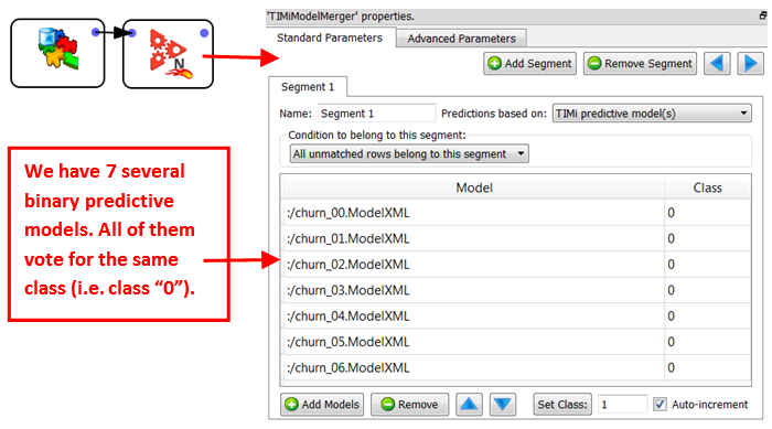
Once again, the final churn probability is the mean (or the median, depending on the settings) of the individual probabilities of each of the 7 models.

 

 
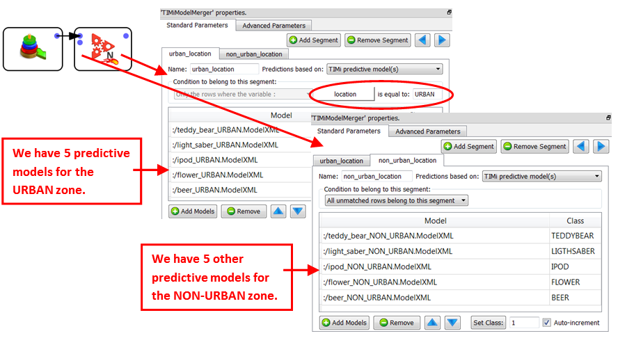
Finally, it’s quite common to create different predictive models for the different segments of your population. For example: it can happen that the purchasing behavior of your customers is totally different depending if the customer resides in an urban zone or not. In such a case, we’ll have 2 sets of models (“urban” and “non-urban”). For example:

 

 

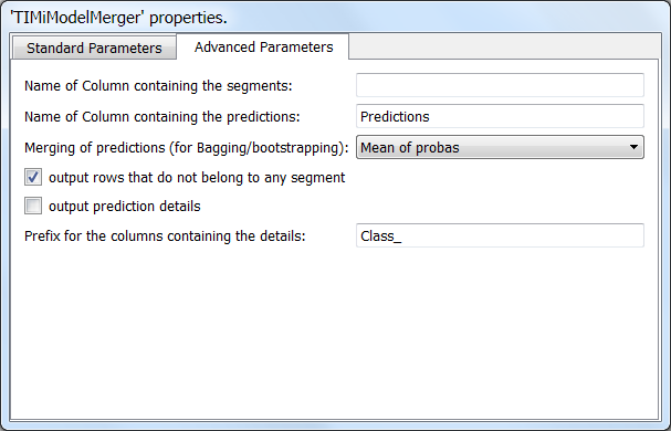
The advanced parameter tab contains some more parameters:

   

 

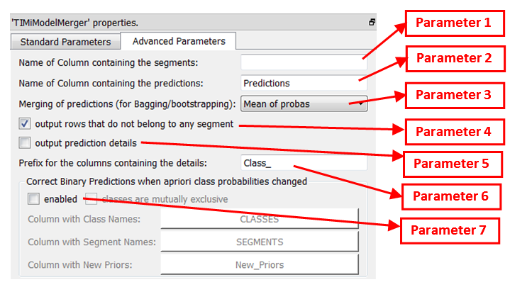
Parameter 1: If this parameter is non-empty, a column containing the segment name (e.g. “urban_location” or “non_urban_location”) is added to the result table.
 

Parameter 2: Name of the column containing the final prediction:
 

•For a binary classification problem, this column contains the ‘final” probability.

•For a continuous prediction problem, this column contains the ‘final” prediction.

•For a Multi-Class classification problem, this column contains the most-likely class (e.g. “TEDDYBEAR”, “LIGTHSABER”, “IPOD”, “FLOWER”, “BEER”).

 
Parameter 3: The operator user to aggregate into one “final” number the individual probabilities given by each predictive model (to obtain the final probability to belong to a specific class).
 

Parameter 4: Self-explanatory

 

Parameter 5: When the parameter “output prediction details” is checked, we’ll obtain:
 

•For a binary or continuous predictive model: Each of the individual probabilities given by each of the predictive models.

•For a multi-class predictive model: The different probabilities to belong to each of the different classes. When using the “1 vs 1” type of predictive models or when using “bagging”, “boosting” or “ensemble learning”, these probabilities are already “aggregated” values of different individual probabilities.

 

Parameter 6: Prefix of the name of the columns containing the “details”. You can change the prefix to avoid any column name collision.

 

Parameter 7: When this option is activated, Anatella computes some corrections on the probabilities computed by the different predictive models to account for the fact that the density of (binary) targets inside the training set(s) is different from the density of targets inside the apply/scoring set. This correction is named, in technical terms, “apriori correction”. To use this option, you must give on the second input pin of this Action, a table that contains the expected density of targets inside the apply/scoring dataset (i.e. the new apriori probabilities) for each different classes&segments. Here is an example:

 

 

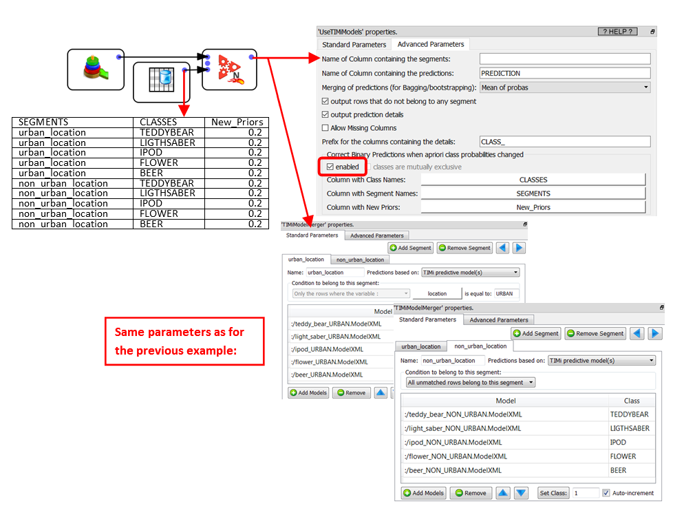
In the above example we corrected the apriori probabilities so that all items (teddy bear, light saber, ipod, flower, beer) have equal apriori’s (i.e. 20%) whatever the percentage of targets that was actually observed in the learning dataset(s) used to create the various predictive models.

 

For even faster deployment of your scoring/models, the TIMiUseModels Action can run inside a N-Way multithreaded section (see section 5.3.2. about multithreading).