|
<< Click to Display Table of Contents >> Navigation: 5. Detailed description of the Actions > 5.12. TA - R Predictive > 5.12.8. Time Series (
|
Icon:
Function: R_timeSeries
Property window:

Short description:
Build and compare TimeSeries
on sequential data
Long Description:
Use this node to compute ETS, STLF, ARIMA and Holt-Winters models.
At the very least, you need to have two series: one with dates (YYYY-MM-dd or YYYY/MM/dd or any separators, as long as the order and number of characters is respected).
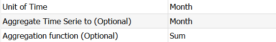
Then, you need to specify the time units between observations (Unit of Time). Anatella will attempt to do it for you, and if it doesn’t match the data, it will recode it. But it’s always better to help the software.
Then, specify on which time frame you wish to run the analysis (Aggregate Time Series) to get smoother – and usually better – results. You can specify whether you want the sum or the average computed
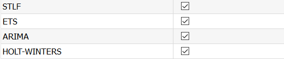
Then, you can optionally uncheck the algorithms you don’t want to run (because you know what you are doing... or leave them all checked and let R figure out which one works.
|
When you run the algorithms, make sure you force anatella to write cache: right click on the object and set the option |
You can set some advanced parameters for the decomposition, for ARIMA and for Holt Winters.
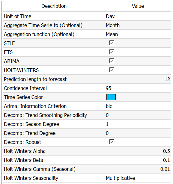
Arima: Information Criterion: By default, you should use BIC as a criterion, as it will perform better if heterogeneity is large (Aho, 2014) , but AIC an AICC are also available and should be checked as other criterion may yield better models. As a reminder, the key difference between AIC and BIC is that BIC penalizes stronger the number of parameters, and this is often desirable.
Consider ![]() is the max likelihood estimates of the model parameters,
is the max likelihood estimates of the model parameters, ![]() is the log likelihood of the model,
is the log likelihood of the model, ![]() is the number of parameters and
is the number of parameters and ![]() the number of observations.
the number of observations.
AIC: Akaike Information Criteria = ![]()
AICC: Aikake for Small Samples ![]()
BIC: Bayesian Information Criteria. ![]()
Thus, when you have few observations (as often in timeseries) AICC would be the most conservative (and preferred) test to apply. When you have “a lot” of points (over 100), BIC or AIC would be appropriate.
The details of the model are available in the log:
Model Information: Series: timeSerie ARIMA (1,0,1) (2,1,0) [12]
Coefficients: arl mal sarl sar2 0.8020 -0.5961 -0.6803 -0.4174 s.e. 0.1671 0.2171 0.0956 0.0995
sigma^2 estimated as 974.6: log likelihood=-526.74 AIC=1063.48 AICc=1064.07 BIC=1076.89
Error measures: ME RMSE MAE MPE MAPE MASE Training set 0.6694643 29.06258 21.78323 -0.4048295 6.963703 0.6720913 ACF1 Training set -0.0313262
Forecasts: Point Forecast Lo 80 Hi 80 Lo 95 Hi 95 Jan 1991 496.5844 456.5766 536.5921 435.3978 557.7710 |
Trend Smoothing Periodicity: this parameter will set how many periods are used to smooth the trend line. If you put a small number, you will have a very non-linear trend, if you put a large number you will get something more stable. If you leave it at 0, the default value of R for (t.window)is used:
nextodd(ceiling((1.5*period)/(1-(1.5/s.window))))
Decomp: Season Degree: (0/1) degree of the function for seasonality. Set to 0 if you don’t think there is seasonality
Decomp: Trend Degree: (0/1) degree of the function for trend. Set to 0 if you don’t think there is trend
Decomp Robust: Set if you want to use a robust method
Holt Winters alpha, Beta and Gamma: Set starting values to help avoid local optima.
Outputs
If you are lucky (you have a data structure that fits the time series framework) you will get the following plot:
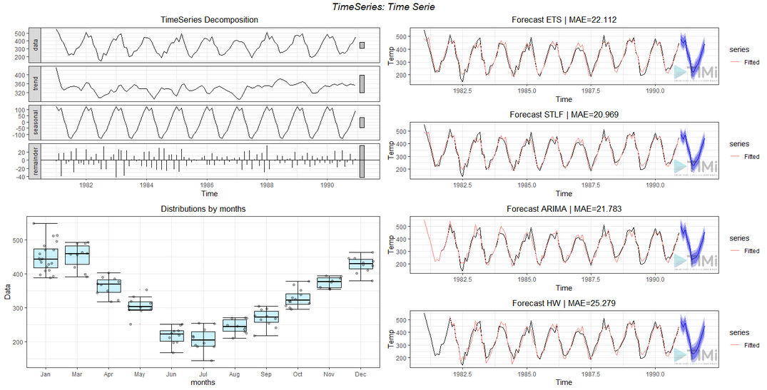
Here, we can observe the decomposition of trend, seasonality and error of the data, a box plot showing the distribution (error) per time unit, and the results of each algorithm.
You can pick the one with the lowest MAE, of look at the diagnostics for more KPIs:
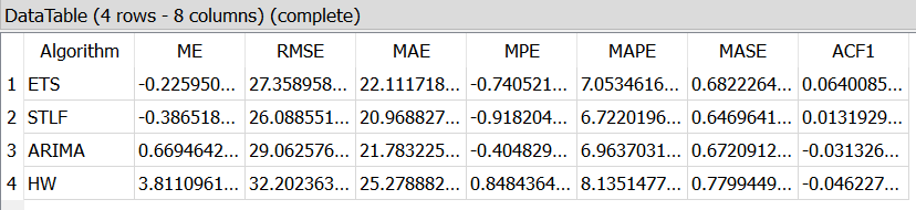
Running... (21/2/22 18:08:13) [1] "Set Time Unit to Days (minimum frequency), StartUnit== 1" ME RMSE MAE MPE ETS -0.225950033418252 27.3589584352165 22.1117188650616 -0.740521333848271 STLF -0.386518286476155 26.0885511361616 20.9688275434863 -0.918204402968769 ARIMA 0.669464278059237 29.0625764891712 21.7832252493945 -0.404829515401513 HW 3.81109616563921 32.2023638385829 25.2788828886824 0.848436419880703 MAPE MASE ACF1 ETS 7.05346168010657 0.682226499093432 0.0640085212331007 STLF 6.72201962179413 0.646964168294057 0.0131929824344223 ARIMA 6.9637031816088 0.672091282977547 -0.0313261956920077 HW 8.13514778925323 0.779944963997742 -0.0462278167592328
Success! (finished at 21/2/22 18:08:25 after 12.04 seconds - Peak Memory Consumption~ 295 MB) |
The same information is available in the second output pin:
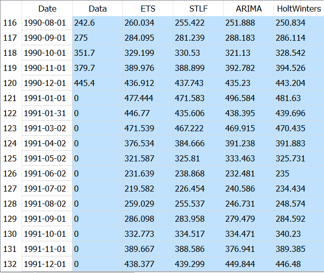
The first output pin will give you the computed estimates for each observation, as well as the prediction for all successful algorithms (for those, the original observation will be set to 0)
If we are unlucky, the time series will fail to decompose, and /or you may end up with constant estimates (when the algorithms doesn’t simply fail). In this case, only the box plot and timeSeries plots will be returned. You will also see and error message in the log telling you what happened (in R dialect)
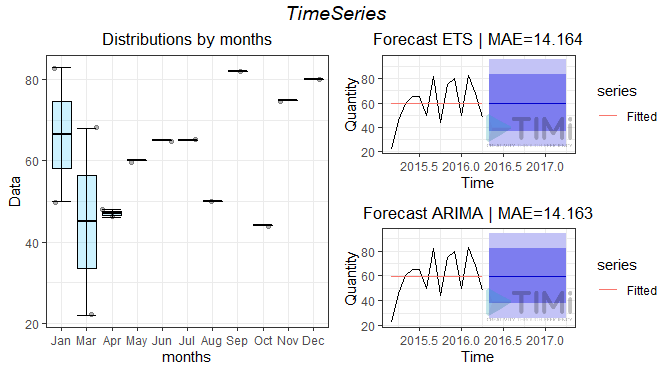
[1] “Error. Failed to converge STLF Algorithm.\nThe R library said:\nError in stl(ts(deseas, frequency = msts[i]), s.window = s.window[i], : series is not periodic or has less than two periods\n" [1] “Error. Failed to converge Holt-Winters Algorithm.\nThe R library said:\nError in decompose (ts(x[1L:wind], start = start(x), frequency = f£), seasonal): time series has no or less than 2 periods\n" [1] "nSeries= 2" [1] “Warning: Failed to decompose TimeSeries. Decomposition not plotted.” <simpleError in stl(timeSerie, s.window = "periodic", t.window = idxPeriod): series is not periodic or has less than two periods> |
In this case, STLF and Holt Winters failed, Arima and ETS failed without crashing, and simply return a constant prediction. The reason here is obvious: there is not enough data to find cycles!