Common database engines (such as Oracle, Teradata, MS-SQL-Server, etc.) have been optimized to be very efficient and fast when you need to:
•Find a particular cell in a large table containing billions of cells.
•Update a few cells in a large table.
These optimizations are adapted to the typical workloads that a database needs to run: Here are some examples of workloads:
•You make a money transfer from your bank account to another bank account. This involves updating (at least) two cells:
oThe first cell contains your current “bank account balance”: i.e. you need to substract from the value stored in this cell the transferred money amount.
oThe second cell contains the destination “bank account balance”: i.e. you need to add the transferred amount to the value that is stored in this cell.
•You purchase a MP3 from a webstore. This also involves updating a very small number of cells/rows. Typically, we’ll have something like:
oUpdate the cell that contains your money balance to substract the value of the purchased MP3.
oAdd one row inside the table that lists which MP3 belongs to which user.
o…and some other small modifications to the webshop database.
•You want to get a list of all the money transfers executed over the last minutes (or seconds). This involves finding a few rows out of a table containing (possibly) billions of rows.
To find the “right” cells to display/process at a very high speed, the database engines are using a data-structure that is named “INDEX”. Typically, if you forgot to add an INDEX to a table inside a database, all the operations on this table will be extremely slow because the database engine will be forced to always do “full table scans” to find the cells/rows required to perform your commands. What’s a “full table scan”? A “full table scan” means that the database engine will be forced to read the whole table (i.e. all the rows from top to bottom in order to find the few cells/rows required to perform your command(s). More precisely, the database engine might be forced to read hundreds of Terabytes out of the hard drive, just to find the one or two cells that needs to be displayed/updated. This is terrible! In opposition, when an INDEX exists, the database uses the INDEX structure to directly find the location (e.g. the offset inside a file containing your table inside your hard drive) of the few cells that are required to perform your commands. Once this location is known, the database engine can then read and/or update the required cells at a very high speed. More precisely, the database engine will read or update a few hundred bytes inside your hard drive. This is much faster than a “full table scan” that involves reading Terabytes of data.
Basically, an INDEX allows you to respond extremely quickly to questions such as: “What are the rows that contains the data from the customer with the ID=”Bob”?”. ..and the answer will be: “These are the row number 101,102,103”. Then, assuming that all the rows in the table have the same size (that we’ll name <RowSize>), the database engine can quickly find the byte-offset of the row 101: The byte-offset is: 101 x <RowSize>. This means that, most of the time, to really benefit from the INDEXing mechanism, the database engine must use a constant “row size”: i.e. All the rows must be stored using the same quantity of bytes. In this way, it’s very easy to find the location/offset of a row inside a file, just knowing the row number.
The “constant row size” is annoying because it means that a column that is declared as a VARCHAR(20) (i.e. a column that contains a string of maximum 20 character long) will always use 20 bytes of storage (we assumed here the “Latin1” encoding, to have 1 byte=1 character), whatever the actual content of the cells. There can be some cells that contains shorter strings (e.g. strings that only have 2 characters) but we still use 20 bytes to store these “short” strings nevertheless (despite the fact that we could store a 2 characters string using only 2 bytes). This obligation of “constant row size” thus produces larger files on the hard drive. On the other hand, this “constant row size” is very handy when you need to update one cell: For example, Let’s assume that:
•I have an “PostalAddress” table that have a column named “StreetName” that is declared as a VARCHAR(20).
•I just moved my home address: My “StreetName” changed from “Baker Street” to “Pennsylvania Avenue”.
My new “StreetName” contains more characters (19>12) but, since I declared “StreetName” as a VARCHAR(20), I still have enough space left to “overwrite” my old “StreetName” with the new one (because 19<20). This means that the “update” operation will be very quick and straightforward (i.e. I just need to overwrite the old data with the new).
To summarize, a “classical” database engine:
•Uses INDEXes on your tables to quickly find the rows/cells required to perform your (SQL) commands.
•To really benefit from the INDEXing mechanism, the database engine must use a constant row size (i.e. all rows must use the same quantity of bytes for storage). A constant row size has some PRO’s and CON’s:
PRO |
CON |
oFaster INDEXing o“Updates” operations are fast & straight forward |
oLarger files (filled with zero’s). oNo data compression algorithms (because, then, each row has a different size, due to the compression). |
INSERTing new rows inside a table that has an INDEX structure is very slow. Indeed, each time you insert a new row inside a table, you must update the INDEX structure to reflect the presence of this new row: This is *very* slow! Please refer to the section 5.27.4.1. about the different “tricks” that you can use to avoid losing time when you need to insert rows inside a table that contains an INDEX (because always updating this INDEX structure after each insertion of one new row consumes a large amount of time).
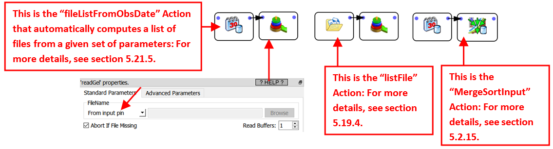
In opposition, the Anatella engine doesn’t keep an INDEX structure on the hard drive (when required, Anatella can actually re-builds an INDEX structure in memory “on-the-fly”: For example, this is what happens inside the ![]() MultiJoin Action or the “In-memory”
MultiJoin Action or the “In-memory” ![]() Aggregate Action). This means that, most of the time, the Anatella engine will be forced to run “full-table-scans”. …but the Anatella engine has been speed-optimized for this situation. When Anatella runs a “full-table-scan” on a table, Anatella need to extract from the Hard drive all the rows from the whole table. So, to go faster, we reduced to the minimum the quantity of bytes required to store the table (extracting less bytes from the hard drive means higher speed): i.e. Inside Anatella, the size of the .gel_anatella files or the .cgel_anatella files is reduced as much as possible: All the cells are as densely “packed” together as possible (in opposition to a database, inside .gel_anatella files there are no “holes”). Anatella uses many different proprietary compression algorithms to reduce the data size. This means that, inside Anatella, it’s not possible to update one cell in the middle of table (if you want to do that, you need to re-create the whole table: i.e. you need to copy the complete .gel_anatella file with a one cell modified). An engine (such as Anatella) that do not have an INDEX structure might seem limited but this has several advantages:
Aggregate Action). This means that, most of the time, the Anatella engine will be forced to run “full-table-scans”. …but the Anatella engine has been speed-optimized for this situation. When Anatella runs a “full-table-scan” on a table, Anatella need to extract from the Hard drive all the rows from the whole table. So, to go faster, we reduced to the minimum the quantity of bytes required to store the table (extracting less bytes from the hard drive means higher speed): i.e. Inside Anatella, the size of the .gel_anatella files or the .cgel_anatella files is reduced as much as possible: All the cells are as densely “packed” together as possible (in opposition to a database, inside .gel_anatella files there are no “holes”). Anatella uses many different proprietary compression algorithms to reduce the data size. This means that, inside Anatella, it’s not possible to update one cell in the middle of table (if you want to do that, you need to re-create the whole table: i.e. you need to copy the complete .gel_anatella file with a one cell modified). An engine (such as Anatella) that do not have an INDEX structure might seem limited but this has several advantages:
•Since the Anatella engine has no INDEX structure, you can add new rows inside your tables (i.e. inside your .gel_anatella or .cgel_anatella files) at a very high speed (i.e. inside Anatella, on a small laptop, you can “insert” in a table several millions rows per second. This is, at least, hundreds times faster than the best databases and, very often, thousands times faster) because you don’t need to maintain and update your INDEX structure at each “INSERT”. It’s thus possible to create very large tables very quickly.
•The overall storage space of your tables is much reduced: Typically, a table stored inside Anatella is from 20 to 100 times smaller than the same table stored inside a classical database because Anatella can “pack & store” the data as efficiently as possible (using advanced compression algorithms) and because Anatella does not lose space to store the INDEX structure.
![]()
The Anatella engine compensates the absence of INDEX by its raw reading (and writing) speed. Indeed, on a common-grade 2000€ laptop, the Anatella engine reads the .gel_anatella files at a speed of about 300 MB/sec (before decompression) or 1GB/sec (after decompressing the data contained inside the file). As a comparison, most databases read their data at a speed of only 10 to 20 MB/sec (because they are forced to read uncompressed data full of “holes”). This makes Anatella run from 50 to 100 times faster than a “classical” database when it comes to pure “reading speed”.
So, despite the fact that the Anatella engine might read out of the hard drive a few more unnecessary rows (because it doesn’t have an INDEX allowing it to avoid reading these rows), it still able to reach very high processing speed because it reads these rows at a very high speed.
This means that Anatella is especially good for jobs that involve reading complete tables (or a very high quantity of row, such as over 90% of the rows of the tables): i.e. Anatella is especially good for jobs that involve “full-table-scans” because these jobs will, typically, run at a speed that is 100 times faster inside Anatella than inside a database.
Since the Anatella engine do not have any INDEXing mechanism, we’ll have to use some “tricks” to avoid reading large tables completely from start to bottom. One very common “trick” is to split our table into many different .gel_anatella files (or .cgel_anatella files). And, thereafter, when you access your table, you extract out of the hard drive only the required files (and we don’t extract/read *all* the small files that are composing the table, otherwise there is no speed gain). In practice, this is done this way:
•TIME-based Splitting:
We’ll assume that each different .gel_anatella file must store the data for a specific day (i.e. we split “by day”). We have inside our original dataset a column named “myDate” that contains the exact day each data-row is linked to. When writing your table on the hard drive, we’ll use the “SPLIT” option of the “writeGel” action in this way:
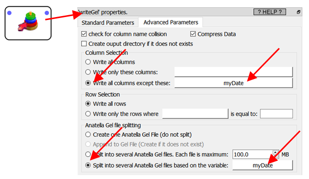
When reading-back the table from the hard drive, Anatella must “assemble” all the different .gel_anatella (one file per day) “as if” there is only one .gel_anatella file (but, in reality, Anatella is concatenating the content of several .gel_anatella). To do so, you can use:
See also the section 5.21.6. for a complete example of “TIME-based Splitting” and databases interaction.
•Key-based splitting
We’ll split our table on a primary key inside your table. This is done this way:
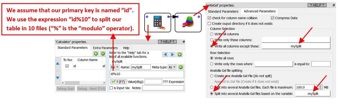
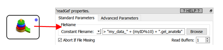
Thereafter, to read the .gel_anatella file that contains the data for a specific “myID” (“myID” is a “graph global parameter”: see section 5.1.5. about “graph global parameters”), we’ll have something like:
As you can guess, the Anatella engine is very good when you have to do “full-table-scans”. “full-table-scans” happens all the time when you do these tasks:
•“Business-Intelligence” Tasks or “Strategic Queries”:
For example: What’s the sum of the revenue for the last 3 months?
We’ll use the “trick” explained hereabove to split the Revenue Table “on time” and only extract/read from the hard drive the .gel_anatella files that are required to compute the sum over the last 3 months. This means that we won’t extract from the hard drive any unnecessary rows (because we only read the .gel_anatella files that matches the requested 3 months and nothing more): i.e. we run a high-speed “full-table-scan” on these files.
To execute “Busines-Intelligence” tasks, the best solution is almost always to run a “full-table-scan”. This means that Anatella is technically the tool that will deliver the highest performances for this type of tasks. In opposition, databases will have comparatively poorer performances (again for this type of “Busines-Intelligence” tasks). This means that Anatella is very often used in conjunction with visualization tools for “Business-Intelligence” (because it’s the fastest&cheapest tool for such tasks). More precisely, Anatella is used to run the heavy aggregations, the heavy “joins”, etc. Once the data size is reduced (i.e. aggregated and cleaned by Anatella) to a smaller, easily manageable size, then you can use practically any vizualisation tool to plot your data. For your convenience, Anatella can directly inject datasets into the most popular data visualization/BI tools:
oAnatella directly creates .hyper files for Tableau (see section 5.27.16)
oAnatella directly creates (and reads back) .qvx/qvd files for Qlik (see section 5.27.17)
oAnatella directly creates .sqlite files for Kibella (see section 5.27.18)
oAnatella directly creates .json files for Kibana (see section 5.27.13)
If your vizualization tool is not listed hereabove, you’ll need to copy your “reduced” datasets inside a classical database for “inter-operability” reasons (because all vizualization tools can access data stored inside a database). See the next section 10.10.2. to know how to make this “copy” procedure as fast as possible. If you are lucky enough to have your vizualization tool listed hereabove, I strongly suggest you to avoid “going through a database” to exchange data with your vizualization tool because the native Anatella connectors are much, much faster (from 10 to 100 times faster).
•“Analytical” Tasks
Very often, the first step of any “Analytical” job is just to create a “Customer View” (also sometime named “CAR : Customer Analytical Record”).
![]()
A “customer view” is a table where each row contain data about a different customer and the columns contains as much as possible different informations about your customers.
Amongst other things, the “Customer View” is used to create optimized marketing campaigns (through predictive analytical and machine learning) and to run many different types of analytics inside a “customer-centric” organization. It’s also used extensively by your CRM system.
Typically, inside a “customer view”, you’ll have a column such as “Number of Puchase over the last Month for this Customer”. To compute this aggregate, you’ll need to read the (very large) “Transaction Table”. And, once again, this translates in technical term to a “full-table scan” (once we used the “trick” explained hereabove to split the Transaction Table “on time”). Actually, to compute all the columns inside the “customer view”, you’ll need to run *many* “full-table scan”. This means that, once again, Anatella is the best tool because it’s technically the tool that will deliver the highest performances because it’s optimized to run “full-table scans”.
Once the “customer view” table is computed, you need to copy it inside your data base, so that other tools can use it (e.g. your CRM system might use your “customer view”). See the next section 10.10.2. to know how to make this “copy” procedure as fast as possible.
•Machine learning, Text Mining, Graph Mining tasks:
These tasks involve creating large tables (that are named in technical terms “Learning datasets”, “Scoring datasets”, etc.). The complete computation of some new tables always involves a “full-table scans” and Anatella is, again, the best technical solution.
The last step of a Machine Learning, Text Mining, Graph Mining, etc. tasks is nearly always to save the new results inside data base (for inter-operability reasons: So that other tools can use these results). See the next section 10.10.2. to know how to make this “copy” procedure as fast as possible.